Model Representation

The basic units: neurons

Biological neuron

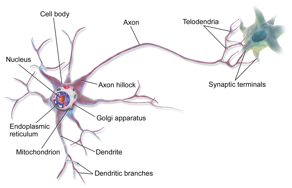
Fig. 40 . Anatomy of a brain cell, the neuron.
_{Source: Wikimedia - BruceBlaus}

As neural networks are inspired from biological brain cells, let’s start with an anatomical introduction. Neurons are each made of a cell body and one long extension called axon, which at the end has ramifications to connect to other neurons’ dentritic branches (around the next neuron cell’s body). The information propagates in the form an electric signal along the axon. At the end of the axon’s branches (telodendria) are synaptic terminals that are terminal structures releasing, depending on the electrical impulse, chemical messengers called neurotransmitters. Those transmitters propagate the information chemically to the next neuron.

Artificial neuron

The first scientists who started to model how biological neurons might work were the neurophysiologist Warren McCulloch and the mathematician Walter Pitts back in … 1943!

Learn More

Let’s go to the source!
If you are curious to read the original paper marking the birth of the artificial neuron:
“A logical calculus of the ideas immanent in nervous activity” - Link on Springer

Definition 52

An artificial neuron is an elementary computational unit of artificial neural networks.

It receives inputs from the dataset or other artificial neurons, combine the information and provide output value(s).

Each input node \(x_j\) is associated with a weight \(w_j\). In terms of components and notations:

• \(x_j\): input nodes

• \(w_j\): weights

• \(b\): bias term

• \(\sum\): weighted sum

• \(f\): activation function

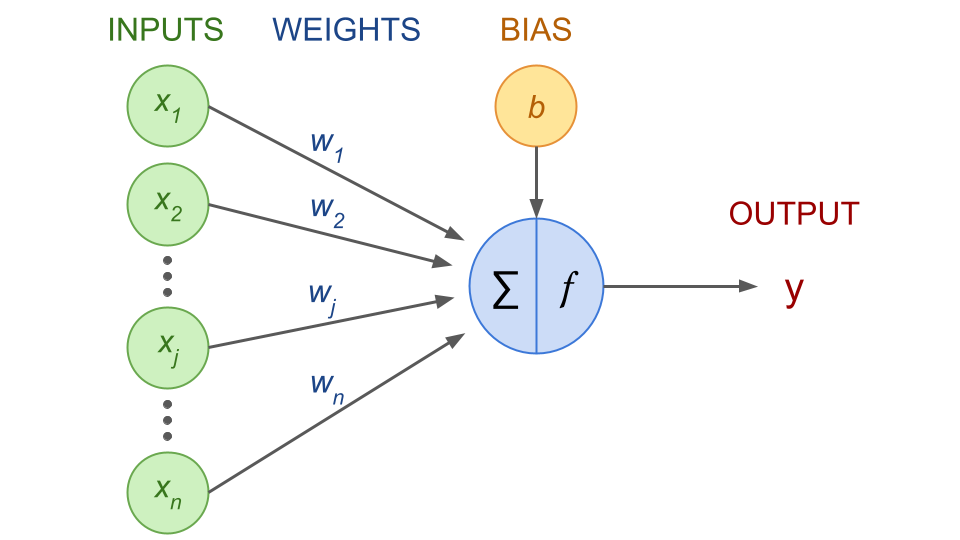
Fig. 41 . Schematics of an artificial neuron. The artificial neuron (center blue) receives \(x_n\) input features and a bias term \(b\). It computes a weighted sum \(\sum\). The activation function \(f\) decides if the neuron is activated, i.e. ‘fires’ the information to the output value \(y\).
_{Image from the author}

Note

The weights of an input node is indicative of the strength of this node.

The bias gives the ability to shift the activation curve up and down. It does not depend on any input.

Now the maths behind a neuron. Recall the linear regression’s sum for the hypothesis function: \(h_\theta(x^{(i)}) = \sum_{j=0}^n \theta_j x^{(i)}_j\). We had an intercept term \(\theta_0\) that was multiplied with \(x_0\), where we assumed by convention that \(x_0 = 1\). We could write it within the sum as we did previously, but in the literature of Neural Networks, it is usually explicitely written outside of the weighted sum from the input nodes (see the comment in the margin). The \(f\) represents the activation function, defined below. So the output of an artificial neuron is given by this key equation:

We used to write \(h_\theta(x)\) for the hypothesis function while computing linear and logistic regression algorithms. It is still valid if we consider \(\theta = ( \boldsymbol{w}, b)\), where \(\boldsymbol{w}\) is a vector of weights \(w_1, w_2, \cdots, w_n\) and \(b\) the bias term (playing the role of \(\theta_0\)). To distinguish notations between regression and neural network, let’s prefer here the notation: \(h_{\boldsymbol{w}, b}(x)\) for the weighted sum.

(50)\[y = f\left(\sum_{j=1}^n w_j x_j + b \right)\]

This operation is done for one sample row \(x^{(i)}\), hence reserving the \(i\) index for the sample instances. The sum is done over the input features \(j\) (columns of the \(X\) input matrix). Here the sum starts at \(j=1\) and not zero as the intercept term is written outside of the sum as \(b\).

We haven’t seen the activation function. Here is its definition:

Definition 53

An Activation Function, also called Transfer Function, is a mathematical operation performed by an artificial neuron on the weighted summed of input nodes (plus the bias node).

As the name indicates, it decides whether the neuron’s input to the network is important or not: returning a non-zero value means the neuron is “activated”, or “fired.”

The purpose of the activation function is to introduce non-linearity into the output of a neural network.

We will see more in details the types of activation functions in the next section.

Now you may wonder how one can compute complex functions with such a simple operating unit. We will see this once we ‘chain’ neurons in different layers. But before that, can one single neuron still be considered a neural network?

Yes it can! And it has a name: it is called the perceptron.

The Perceptron

Definition 54

A Perceptron is a neural network based on a single specific artificial neuron called a Threshold Logic Unit (TLU) or Linear Threshold Unit (LTU), where the activation function is a step function.

It computes a weighted sum of real-valued inputs, has a bias term in the form of an extra node and yield the output:

\[\begin{equation*} h_{\vec{w},b} = \text{step} \left( w^T x + b \right) \end{equation*}\]

A perceptron is thus a linear binary classifier.

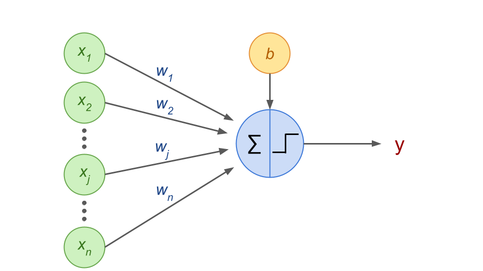
Fig. 42 . Schematics of a perceptron.
_{Image from the author}

The step functions generally employed are the Heaviside or the sign functions:

(51)\[\begin{split}\forall \: z \in \mathbb{R}, \: \: H(z) = \begin{cases} \;\; 1 & \text{ if } z \geq 0 \\ \;\; 0 & \text{ if } z < 0 \end{cases}\end{split}\]

(52)\[\begin{split}\forall \: z \in \mathbb{R}, \: \: {sign}(z) = \begin{cases} \;\; +1 & \text{ if } z>0 \\ \;\;\; 0 & \text{ if } z=0 \\ \;\; -1 & \text{ if } z<0 \end{cases}\end{split}\]

If a perceptron would use the sigmoid as activation function, it would be specified as sigmoid perceptron.

The linear and logistic regression, introduced in Lecture 2 and 3 respectively, can be also achieved by this neuronal animal presented just above. Yet there are core differences between the regression algorithms and the perceptron.

Warning

While linear and logistic regression outputs results that directly be converted to a probability value, the perceptron does not output a probability!
It makes predictions based on a hard threshold.

The perceptron with one logic threshold neuron can, using the step function, split the data into 2 classes depending on its output value exceeding the threshold (predicted class \(y=1\)) or not (\(y=0\)). Think of the perceptron as more a ‘yes’ or ‘no’ system, and logistic regression as “I think it is 67% probable to be the class \(y=1\).”

With one output node, a perceptron can classify from two classes. A perceptron with \(k\) output nodes can classify from \(k+1\) classes. The extra class being encoded as “all outputs not activated,” i.e. \(y_1 = y_2 = y_k = y_n = 0\), would mean the event belongs to class \((k+1)^\text{th}\). It is similar in probabilities when we take:

\[p(N) = 1 - \sum_{i=1}^{N-1} p_i\]

to get the remaining probability in the last outcome possible (but bare in mind that perceptrons do not output probabilities).

Limitation and… abandon

It turned out that perceptrons disappointed researchers. The main limitation: perceptrons can only solve linearly separable data. In other words, it can classify the data if only one can draw a line (or plane with 3 inputs) separating the two classes. While perceptrons can successfully perform the basic logical computations (also called ‘gates’) AND, OR and NOT, it is incapable of solving the trivial XOR problem:

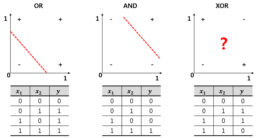
Fig. 43 . The XOR is an exclusive OR (true if only the two logical inputs are different). As the data is not linearly separable, a perceptron is unable to solve it.
_{Image: extsdd.tistory.com}

Moreover, the perceptron doesn’t scale well with massive datasets. Other weaknesses of Perceptrons were highlighted in the monograph Perceptrons by computer scientists Marvin Minsky and Seymour Papert in 1969. The book sparked a wave of pessimism and long-standing controversy in the Artificial Intelligence community (barely born), to the point that some researchers were so disappointed that they dropped neural networks altogether. This is known as the AI Winter. Interest in neural networks was revived only in the mid 80s.

Exercises

1. What would be the weights \(w= (w_1, w_2)\) and bias \(b\) to encode the AND function above? (using the Heaviside step function)

2. Same question for the OR function.

3. Compare your answers with your peers. Are they the same?

Check your answers

Answer 1.
Possible answer:
\(b = -1\)
\(w_1 = 0.5\)
\(w_2 = 0.5\)

Answer 2.
Possible answer:
\(b = -0.5\)
\(w_1 = 1\)
\(w_2 = 1\)

Connecting artificial neurons

Layers

Now that we saw the artificial neuron, let’s see how they can model complex data patterns while connecting them. Like their organic counterparts where neurons are organized in consecutive layers, artificial neural networks are arranged in layers, where neurons in each layer receive input from the previous layer and pass their output to the subsequent layer.

Definition 55

An artificial neural network is composed of:

• input layer: one entry layer of input nodes, i.e. input features from the dataset

• output layer: one final layer of output nodes

• hidden layer(s): one of more layers of nodes called “activation units”

Every layer except the output layer include a bias neuron and is fully connected to the next layer.

Each neuron (or node) performs a linear transformation on the inputs (weighted sum) followed by a non-linearity (the activation function).

Deep or not deep: is that a question?

Definition 56

The number of hidden layers is an indicator of the depth of a neural network.

A ‘minimal’ multilayer neural network would have one input, one hidden and one output layers. The term used is shallow, by opposition to deep. Stricly speaking , or rather historically from the first development in the 1990s, neural networks containing more than one hidden layers are considered deep. Deep Neural Networks (DNN) are also called Deep Nets for short. There is a bit of fuzziness when it comes to what we can consider deep, as nowadays it is common to see dozens of hidden layers.

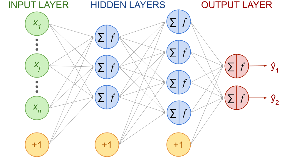
Fig. 44 . Example of a fully connected, feedforward neural network with 2 hidden layers and output size of 2. Bias neurons are represented in yellow circles with +1.
_{Image from the author}

The example of network depicted above is one of the earliest types of neural network and is called a Multilayer Perceptron (MLP). It belongs to a class of neural networks known as feed-forward neural networks, where the information flows only from inputs to outputs (without any loops).

We will see soon how the ouputs of nodes from a given layer is calculated knowing the nodes’output of the previous layer (feedforward propagation). But let’s first have a look of the different activation functions available on the machine learning market in the next section.