Gradient Descent in 1D

Model representation

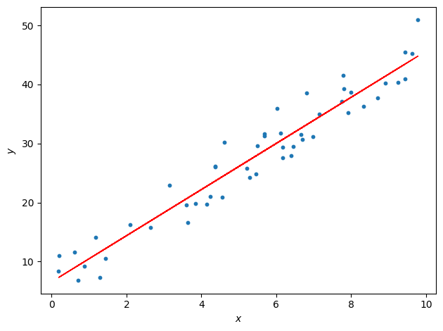
We will study the following situation where we want to predict a real-valued output \(y\) based on a collection of input values \(x\) that would be spread in the following way:

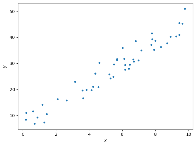
Now I see what you are thinking: it’s very straightforward (pun intended), it is just about fitting a straight line to the data. Yes. But this over-simplified setup is the starting point of our machine learning journey as it contains the basic mathematical machinery. Things will complicate soon, don’t worry.

So, what is linear regression to start with?

Definition 3

Linear regression is a model assuming a linear relationship between input variables and real-valued output variables.

• Input variables are called independent variables, or explanatory variables.

• The output variable is considered a dependent variable.

Linear regression is used to predict a real-valued output variable (dependent variable) based on the values of the input variables (independent variables).

Definition 4

• If there is one explanatory variable, this is simple linear regression or univariate linear regression.

• In the case of several explanatory variables, it is called multiple linear regression.

Let’s now introduce terms more specific to the machine learning jargon and define some notations we will use through the course.

Terminology and Notation

• The input variables are called features and are denoted with \(x\).

• The output variable is the target and is denoted with \(y\).

• In supervised learning the dataset is called a training set.

• The number of training examples is denoted with \(m\).

• The \(i^{th}\) example is \((x^{(i)} , y^{(i)})\).

So the pair \((x^{(1)} , y^{(1)})\) is the first training example from the data set, and \((x^{(m)} , y^{(m)})\) is the last.

Warning

Here we start counting from one. When you will write code, the convention is to start at index zero. So your last sample will be of index m - 1. Keep this in mind.

When we refer to the entire list of all features and targets, we will use, \(x\) and \(y\) respectively. Those are vectors.

We defined the input and output. In the middle is our model. We feed it first with all the input features and their associated known targets. This first step of supervised learning is called the training and we will see the mathematics behind it now. What we need first is a function that best maps input to output.

Definition 5

The hypothesis function, denoted \(h\), is a mapping function used to predict an output \(y\) from an input \(x\):

\[\begin{equation*} y = h(x) \end{equation*}\]

In our simple case of linear regression, our function \(h\) will be of the form:

(1)\[ h_\theta(x) = \theta_0 + \theta_1 \; x\]

The subscript \(\theta\) means that the function depends on the values taken by \(\theta_0\) and \(\theta_1\).

Definition 6

The mapping function’s internal variables are called the model parameters. They are denoted by the vector \(\theta\):

\[\begin{equation*} \boldsymbol{\theta} = \begin{pmatrix} \theta_0 \\ \theta_1 \\ \\ ... \\ \\ \theta_n \\ \end{pmatrix} \end{equation*}\]

In our case with the linear regression with one input feature, we only need two parameters:

(2)\[\begin{split}\boldsymbol{\theta} = \begin{pmatrix} \theta_0 \\ \theta_1 \\ \end{pmatrix}\end{split}\]

We want to find the values of \(\theta_0\) and \(\theta_1\) that fit the data well. We could pick one training example \((x^{(k)} , y^{(k)})\) and derive the coefficients from there. But will this be the ‘best’ straight line to draw? The mathematical phrasing for such a task is to think in terms of errors. How do we calculate the errors? That’s a first question to ask. From a given vector of \(\theta\), how small are the errors? This picture below helps to visualize. From a given parameterization, that is to say a given tuple (\(\theta_0\) , \(\theta_1\) ), the mapping function will output continuous values of a predicted \(y\) for a continuous range of \(x\). That is the dashed line. The errors are the (vertical) intervals between the \(y\) from the prediction and each data points.

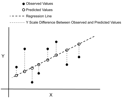
Fig. 9 . Visualization of errors (dotted vertical lines) between observed and predicted values.
Image: Don Cowan.

To see how well the prediction fit the data, we want the sum of all these errors to be as small as possible. In other words, we want to solve a minimization problem.

To avoid cancellation between positive and negative error values, we take the square of each distance; we get a positive number each time that will add up to the total error. Such evaluation is very similar to what is done for the minimum chi-square estimation. The name “chi” comes from the Greek letter \(\chi\), commonly used for the chi-square statistic. We will follow this protocol but in the ‘machine learning way,’ introducing a key concept: the cost function.

Cost Function in Linear Regression

The accuracy of the mapping function is measured by using a cost function.

Definition 7

The cost function in linear regression returns a global error between the predicted values from a mapping function \(h_\theta\) (predictions) and all the target values (observations) of the training data set.

The commonly used cost function for linear regression, also called squared error function, or mean squared error (MSE) is defined as:

(3)\[ J\left(\theta_0, \theta_1\right) =\frac{1}{2 m} \sum_{i=1}^m\left(h_\theta(x^{(i)})-y^{(i)}\right)^2\]

You can recognize the form of an average. The factor \(\frac{1}{2}\) is to make it convenient when taking the derivative of this expression. In Equation (3), each \(h_\theta (x^{(i)})\) is the prediction with our mapping function, whereas \(y_i\) is the observed value in the data.

The initial goal to “fit the data well” can now be formulated in a mathematical way: find the parameters \(\theta_0\) and \(\theta_1\) that minimize the cost function.

(4)\[\min_{\theta_0, \theta_1} J\left(\theta_0, \theta_1\right)\]

Let’s simplify for now the problem by assuming the following data set:

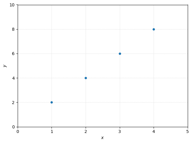
This is an ideal case for pedagogical purposes. What are the values of \(\theta_0\) and \(\theta_1\) here?

Check your answers

Recall the mapping function for linear regression: \(h_\theta(x) = \theta_0 + \theta_1 x\). As we have a correspondance \(y = 2x\) for all points, so \(h_\theta(x) = 2x\), so \(\theta_0 = 0\) and \(\theta_1 = 2\).

You will appreciate the simplification, as we will calculate the cost by hand for different values of \(\theta_1\). More complicated things await you in the tutorial, promised.

Exercise

• Start with a value of \(\theta_1\) = 1 and calculate the cost function \(J(\theta_1)\).

• Proceed the same for other values of \(\theta_1\) of 0.5, 1.5, 2, 2.5, 3.

• How would the graph of the cost function \(J(\theta_1)\) as a function of \(\theta_1\) look like?

• Are there maxima/minima? If yes how many?

Solutions | Don’t look too soon! Give it a try first.

The values of the cost function for each \(\theta_1\) are reported on the plot below:

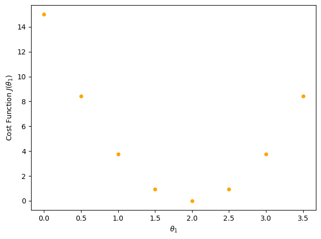
We see that in this configuration, as we ‘swipe’ over the data points with ‘candidate’ straight lines, there will be a value for which we minimize our cost function. That is the value we look for (but you will learn to make such fancy plot during the tutorials).

This was with only one parameter. How do we proceed to minimize with two parameters?

Visualizing the cost

Let’s see a visual representation of our cost function as a function of our \(\theta\) parameters. We saw in the simple example above that the cost function \(J(\theta_1)\) with only one parameter is a U-shaped parabola. The same goes if we fix \(\theta_1\) and vary \(\theta_0\). Combining the two, it will look like a bowl. The figure below is not made from the data above, just for illustration:

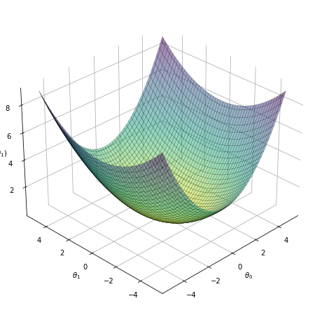
Fig. 10 . The cost function (vertical axis) as a function of the parameters \(\theta_0\) and \(\theta_1\).

What does this represent? It shows the result of the cost function calculated for a range of \(\theta_0\) and \(\theta_1\) parameters. For each coordinate (\(\theta_0\) , \(\theta_1\)), there has been a loop over all the training data set to get the global error. The vertical value shows thus how ‘costly’ it is to pick up a given (\(\theta_0\) , \(\theta_1\)). The higher, the worse is the fit. The center of the bowl, where \(J(\theta_0 , \theta_1)\) is minimum, corresponds to the best choice of the \(\theta\) parameters. In other words: the best fit to the data.

How do we proceed to find the \(\theta_0\) and \(\theta_1\) parameters minimizing the cost function?

Gradient Descent

This concept is key in machine learning. We will see the procedure with our example. But first of all, what is gradient descent?

Definition 8

Gradient descent is an iterative optimization algorithm to find the minimum of a function.

The 3D plot above is misleading, as we will see that once we add input features we cannot have any visual of how the data landscape looks like (we are stuck with 3D vision, rarely 4D and that’s it). In a way, we are blind. Think of yourself walking from a point of the bowl-shaped surface but in the dark. How to reach the ‘valley’ where the cost function is minimum?

The idea behind gradient descent is to walk step by step following the slope of the cost function locally. In mathematical words: the partial derivatives of the cost function will give us the best direction to go towards the minimum.

Terminology

Hyperparameter
A model argument set before starting the machine learning algorithm.
Hyperparameters control the learning process.

Learning rate \(\alpha\)
Hyperparameter in an optimization algorithm that determines the step size at each iteration while moving toward a minimum of a loss function.
The learning rate is always a strictly positive number.

Epoch
In machine learning, an epoch is the number of passes of the entire training dataset the machine learning algorithm has completed.
The number of epochs is a hyperparameter controlling the number of passes of the algorithm.

The steps of the gradient descent algorithm for a linear regression with two parameters (i.e. in 1D) are written below.

This definition will be generalized in the next section with more parameters, from \(\theta_0\) to \(\theta_n\).

Algorithm 1 (Gradient Descent for Univariate Linear Regression)

Inputs

• Training data set with input features \(x\) associated with their targets \(y\):

\[\begin{equation*} x = \begin{pmatrix} x^{(1)} \\ x^{(2)} \\ \vdots \\ \\ x^{(m)} \end{pmatrix} \hspace{10ex} y = \begin{pmatrix} y^{(1)} \\ y^{(2)} \\ \vdots \\ \\ y^{(m)} \end{pmatrix} \end{equation*}\]

Hyperparameters

• Learning rate \(\alpha\)

• Number of epochs \(N\)

Outputs
The optimized values of the parameters: \(\theta_0\) and \(\theta_1\), minimizing \(J(\theta_0 , \theta_1)\).

1. Initialization: Set values for \(\theta_0\) and \(\theta_1\)

2. Iterate N times or while the exit condition is not met:

   1. Derivatives of the cost function:
      Compute the partial derivatives of \(\frac{\partial }{\partial \theta_0} J(\theta_0 , \theta_1)\) and \(\frac{\partial }{\partial \theta_1} J(\theta_0 , \theta_1)\)

   2. Update the parameters:
      Calculate the new parameters according to:

   (5)\[\begin{split}\begin{align*} &\\ \theta'_0 &= \theta_0-\alpha \frac{\partial}{\partial \theta_0} J\left(\theta_0, \theta_1\right) \\ \\ \theta'_1 &= \theta_1-\alpha \frac{\partial}{\partial \theta_1} J\left(\theta_0, \theta_1\right) \end{align*}\end{split}\]

            Reassign the new \(\theta\) parameters to prepare for next iteration

(6)\[\begin{split}\begin{align*} \theta_0 &= \theta'_0 \\ \\ \theta_1 &= \theta'_1 \\ \end{align*}\end{split}\]

Exit conditions

• After the maximum number of epochs \(N\) is reached

• If both derivatives of the cost function \(\frac{\partial}{\partial \theta_0} J\left(\theta_0, \theta_1\right) = \frac{\partial}{\partial \theta_1} J\left(\theta_0, \theta_1\right) = 0\)

In linear regression, the partial derivatives can be simplified.

Exercise

Knowing the form of the hypothesis function \(h_\theta(x)\) for linear regression and the definition of the cost function, rewrite the Equation (5) with the explicit partial derivatives.

Answer

\[\begin{align*} \theta'_0 &= \theta_0-\alpha \frac{1}{m} \sum_{i = 1}^m \left(h_\theta(x^{(i)})-y^{(i)}\right) \\ \\ \theta'_1 &= \theta_1-\alpha \frac{1}{m} \sum_{i = 1}^m \left(h_\theta(x^{(i)})-y^{(i)}\right) x^{(i)} \end{align*}\]

Details on demand during office hours.

Important
Note that at the step 2.1., there is an implicit loop over all training data samples, as it is required by the cost function.

Why a minus sign before alpha?
This illustration helps see why the minus sign in Equation (5) is necessary.

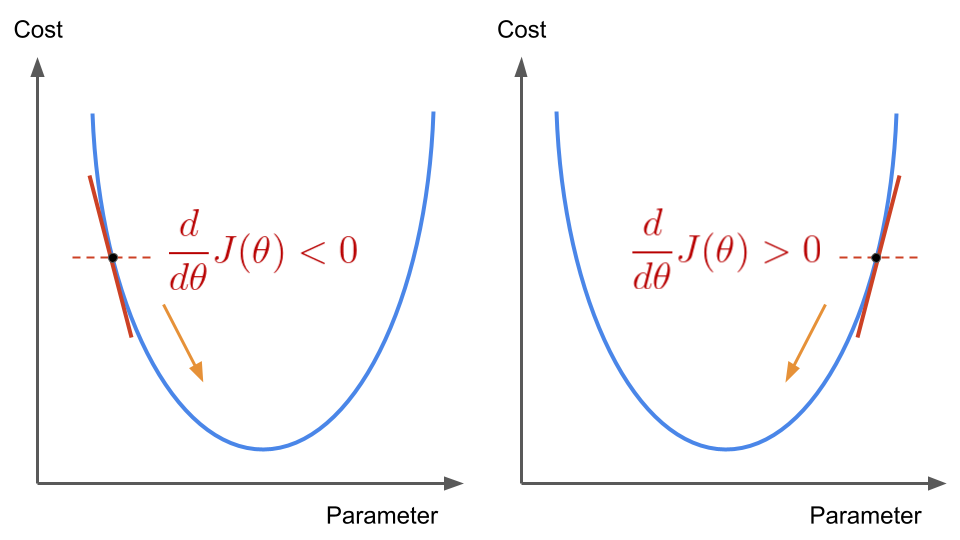
Fig. 11 . The sign of the cost function’s derivative changes for two different parameter values either lower (left) or greater (right) than the parameter value for which the cost function is minimized.
_{Image from the author}

If our parameter is randomly picked on the left side of the U-shaped parabola, the partial derivatives will be negative. As the learning rate is always positive, the incremental update \(-\alpha \frac{d}{d \theta} J(\theta)\) will thus be positive. We will add an increment to our parameter. At the next iteration, we will have a new parameter \(\theta\) closer to the one we look for. The reverse goes with the other side of the curve: with a positive derivative, we will decrease our parameter and slide to the left. All the time we go ‘downhill’ towards the minimum.

Graphical Visualization of the Gradient Descent

When computing the gradient descent for linear regression, we get new parameters so we can draw a candidate straight line to fit the data. With proper tuning (more on this later), we reach the ideal fit, minimizing the cost function.

Fig. 12 . Animation of the gradient descent. At each generation a new set of parameters are computed. In this picture \(m\) corresponds to \(\theta_1\) and the constant \(c\) to \(\theta_0\). Sometimes they are also referred to the slope and intercept respectively.
_{Source GIF: Medium}

In our example, the best linear fit will be:

How to picture this in the \(\theta\) parameter space? For this, contour and 3D plot are handy. Below, the new parameters’trajectory (red points) are “descending” towards the minimum of the cost function:

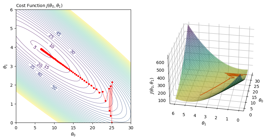
Fig. 13 . Contour plot (left) and 3D rendering (right) of the cost function with respect to the values of the \(\theta\) parameter. The red dots are the intermediary values of the parameters at a given iteration of the gradient descent. You can see that it converges toward the minimum of the cost function.

We will discuss the presence of the zig-zag behaviour in the first iterations in section Learning Rate.

This was linear regression with one input feature. Let’s move on with a more generalized version of linear regression involving multiple features.