What are Decision Trees?
Contents
What are Decision Trees?#
Without knowing, you may have already been implementing a ‘decision tree’ process while making a choice in your life. For instance, which cereal box to buy at the store. There are so many brands and options (understand classes) that it can be overwhelming. Here is a tree-like reasoning example:
Does it have more than three types of flakes? No? Too boring. Yes? Let’s move on:
Is a portion bigger or lower than 300 calories? Bigger? It’s not healthy, let’s go lower and see the next parameter:
Is it crunchy? If yes, I take that one!
Your decision protocol followed a tree process starting with a node (a decision to make), then evaluating a condition on a feature (number of flake type, calorie density, crunchiness factor) and, depending on the answer, another node evaluates another input feature. Such a decision-making process can be visualized like a tree whose branches are the different outcomes and leaves the final choices:
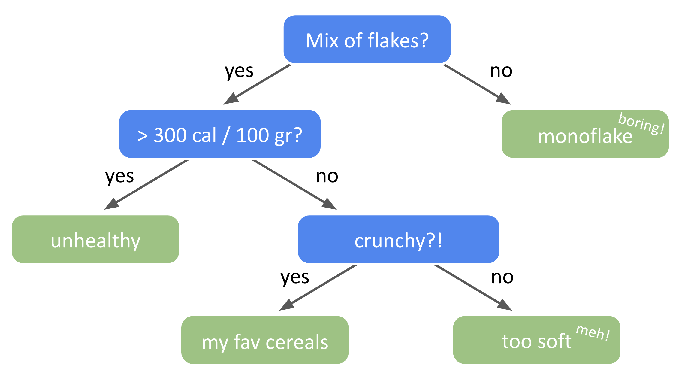
Fig. 32 . An example of decision tree for how to choose cereals.
Image by the author#
Decision trees belong to the family of machine learning algorithms for both classification and regression (we will focus on classification here).
Definition#
Definition 40
A decision tree is a flowchart mapping a decision making process. It is organized into nodes, branches and leaves.
Definition 41
A tree consists of three types of nodes:
Root node: The start of the decision process is the first test performed on the whole dataset.
Internal nodes: A “condition box” evaluating subset of the dataset on a given feature. The test has two possible outcomes: true or false.
Leaf nodes or terminal nodes: Nodes that do not split further, indicating – most of the time – the final classification of data points ‘landing’ in them.
The outcomes of that evaluation (either boolean or numerical) is divided into branches, or edges. Each branch supports one outcome (usually True/False) on the condition from the previous node.
Example#
Let’s illustrate the terminology with an example. Let’s have a dataset with two variables as input features, \(x_1\) and \(x_2\).
    from sklearn.tree import DecisionTreeClassifier

    tree_clf = DecisionTreeClassifier(max_depth = 2)
    tree_clf.fit(X, y)
The code has been shortened for clarity, see the notebook for completeness.
To visualize the work of the decision tree classifier, the graphviz library creates an automated flowchart:
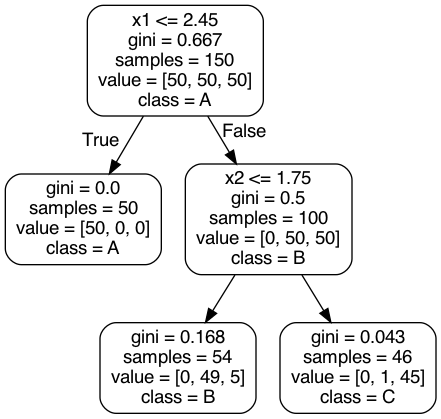
Fig. 33 . Example of a Decision Tree drawn from sklearn pre-loaded dataset iris. The root node is at the top, at depth zero. The tree stops at depth = 2 (final leaves).#
Such a flowchart above tells how future predictions are made. Predicting the class of a new data point (\(x_1^\text{new}\), \(x_2^\text{new}\)), one simply follows the ‘route’ of the tree starting from the root node (on top) and ‘answering’ the conditions. Is \(x_1\) lower than 2.45? Yes, go to the left (and it corresponds to predicted class A). If not, go to the next node evaluating \(x_2\) feature, etc.
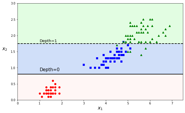
The predictions can be visualized on a 2D scatter plot. The threshold values are the decision boundaries (see Definition 18 in section What is the Sigmoid Function?) and are materialized by either vertical or horizontal cuts. Instead of a straight line or polynomials fit, a decision tree rather makes an orthogonal segmentation of the phase space.
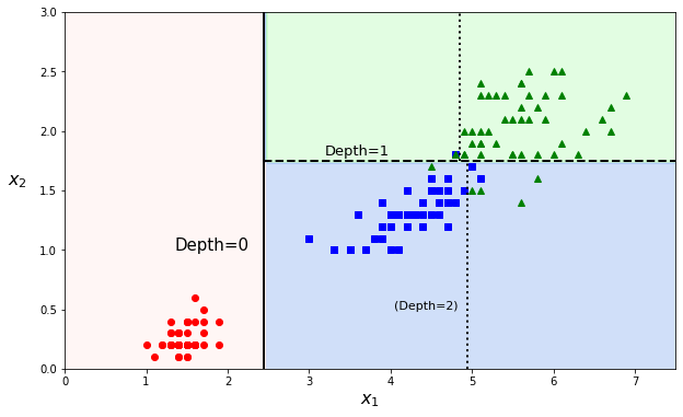
The first node at depth 0 creates a first decision boundary, splitting the dataset into two parts (and luckily isolating class A in a pure subset). The second cut is at depth 1. As the tree was set to a max depth of 2, the splitting stops at depth 1 (as we start from zero). But it is possible to continue further with a max depth of 3 and the decision boundaries (several for each branch) would be the dotted vertical lines.
We could see with an example and illustrative graphs how the decision tree splits the datasets. But how are these splits calculated? Why did the classifier chose the cut values \(x_1\) = 2.45 and \(x_2\) = 1.75? This is what we will cover in the following section.
Algorithm#
There are metrics entering in the optimization algorithm of a decision tree. The main one is the Gini impurity:
Definition 42
The Gini’s diversity index is a measure of a node’s impurity.
It is defined for each tree node \(i\) as:
with \(N_{k, i}\) the number of data samples of class \(k\) in node \(i\) and \(N_{i}\) the total number of data samples in node \(i\). The terms \(p_k\) in the sum are equivalent to the probability of getting a sample of class \(k\) in the node \(i\).
The Gini’s impurity index ranges from 0 (100% pure node) to 1 (very impure node).
If a node has an equal amount of data points from two classes, let’s say 500 points each, the Gini index will be:
With three classes present in equal quantities, it will be \(\frac{2}{3}\), for four, \(\frac{3}{4}\), etc.
The algorithm used for classification trees is called CART. It stands for Classification and Regression Tree. Once again, we will need a cost function to minimize. This cost function will be defined at a given node containing \(N_\text{node}\) data samples.
Definition 43
The cost function for CART is defined as:
It is a sum where the purity of each subset is weighted by the subset sizes. In the literature, you may see the terms left and right. They translate as:
left: all data points whose feature \(x_j\) is such that \(x_j < t_j\)
right: all data points whose feature \(x_j\) is such that \(x_j \geq t_j\)
We will see the role of the hyperparameters later. This is for now the pseudocode:
Algorithm 3 (Classification and Regression Tree)
Inputs
Training data set \(X\) of \(m\) samples with each \(n\) input features, associated with their targets \(y\)
Hyperparameters
Max Depth
Minimum sample split
Minimum samples per leaf,
Maximum leaf nodes
…
Outputs
A collection on decision boundaries segmenting the \(j\) feature space.
Initialization: at the root node
STEP 1: THRESHOLD COMPUTATION:
For each feature \(j\) from 1 to \(n\):
\(\;\;\;\) For a value of \(t_j\) scanning the range \(x^\text{min}_j\) to \(x^\text{max}_j\):
\(\;\;\;\;\;\; \rightarrow\) Compute the cost function \(J(j, t_j)\)
\(\;\;\;\;\;\; \rightarrow\) Find the pair \((j, t_j)\) that produces the purest subsets, i.e. so that it minimizes:
STEP 2: BRANCHING:
Split the dataset along the feature \(j\) using the threshold \(t_j\) into two subsequent new nodes.
Repeat Step 1 at each new node.
Exit conditions
At least one condition on one of the hyperparameters is fullfilled
One of the greatest strength of decision tree is the fact very few assumptions about the training data are made. It differs from linear or polynomial models where we need to know beforehand that the data can be fit with either linear or polynomial function.
Another advantage: feature scaling is not necessary. No need to standardize the dataset beforehand.
Decision trees are also easy to interpret. It’s possible to check calculations and apply the classification rules even manually. Such clarity in the algorithm, often called white box models, contrasts with the black boxes that are for instance neural networks.
Despite these advantages, decision trees have several limitations.
Limitations#
Cutting down on overfitting#
Decision trees are choosing the cut values solely on the available dataset. If let unconstrain, they will continue their way cutting through the data noise, ineluctably leading to overfitting. The way to regularize them is done through the hyperparameters, restricting their freedom:
maximum depth is stopping the algorithm after the node ‘depth - 1’ (as the starting node is zero)
minimum sample split is the minimum number of samples a node must have before it can be split
minimum sample leaf restricts the number of samples within a leaf, preventing an over-segmentation of the data into small square ‘islands’ with very few data samples in them
maximum leaf nodes is an upper bound on the amount of leaves (final nodes)
Exercise
How to tweak (increase of decrease) the hyperparameters in order to relevantly perform a regularization?
Check your answers
Hyperparameters with a minimum should be increased and those with a maximum bound should be decreased in order to regularize the decision tree.
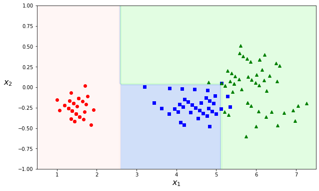
Orthogonal cuts#
As the decision trees work with threshold values, the boundaries are always perpendicular to an axis. This works well if the data is ‘by chance’ aligned with the axes. This ‘feature’ makes decision trees sensitive to rotation. If we rotate the dataset used in the example above, we can see it changes decision boundaries:
angle = np.pi / 180 * 20
rotation_matrix = np.array([[np.cos(angle), -np.sin(angle)], [np.sin(angle), np.cos(angle)]])
Xr = X.dot(rotation_matrix)

tree_clf_r = DecisionTreeClassifier(random_state=42)
tree_clf_r.fit(Xr, y)

plot_decision_boundary(tree_clf_r, Xr, y, axes=[0.5, 7.5, -1.0, 1])
Instability#
Not only rotated data samples, decision trees can also drastically change with only minimal modification in the data. Removing one data point in the dataset above can lead to very different decision boundaries:
Instability will change future predictions and is quite a bad feature (bug) from a machine learning algorithm. How to circumvent this intrinsic instability? This is what we will cover in the next section!