What is the Sigmoid Function?

General definition

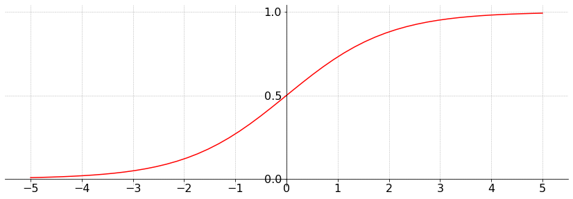
A sigmoid function refers in mathematics to a category of functions having a characteristic “S-shape” curve. Among numerous examples, the one commonly used in machine learning is the logistic function.

To avoid confusion with the fact we already use \(x\) for the input features, the input variable in the definition opposite is written with another letter, \(z\).

Definition 16

The logistic function is defined for \(z \in \mathbb{R}\) as

\[\begin{equation*} f(z) = \frac{1}{1 + e^{-z}} \end{equation*}\]

It looks like this:

A better mapping

In our example with the energy of the electron, we could see from the data (easily because it is only in one dimension) that the bigger the energy of the electron, the more likely it is for the event to be classified as signal. If we overlay the S-curve on the data points, we start seeing interesting things.

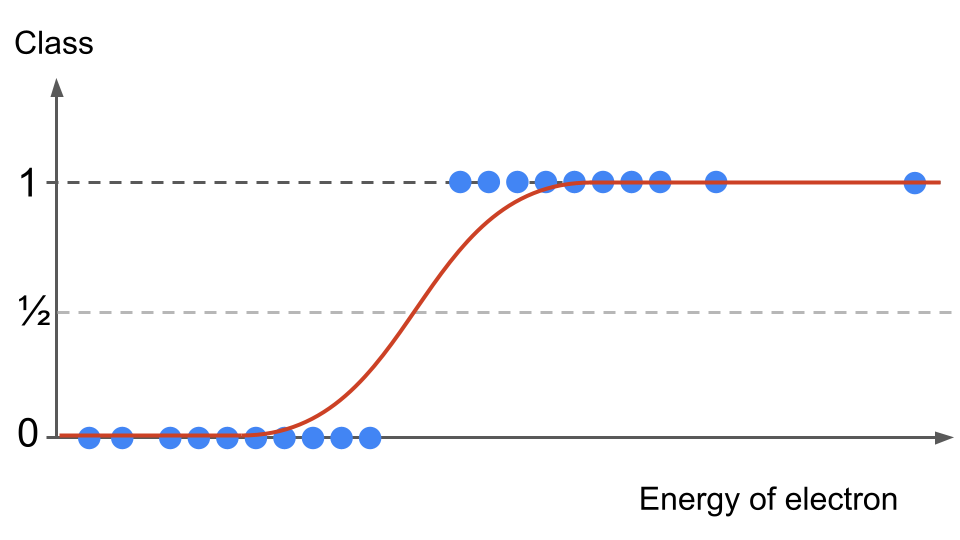
Fig. 19 . Data 1D distribution and sigmoid overlaid

First of all, the curve is not overshooting below or above our discrete outcomes’ range. Second: for data points either far left or far right, instead of creating a large error with a straight line as previously, the S-curve actually takes the values of our target-variables (asymptotically). Consequence: the error between the prediction and observed values will be very small, even negligible. We will not have an unwanted shift and mis-classification like before.

Sigmoid function for logistic regression

Definition 17

A mapping function \(h_\theta(x)\) used for logistic regression is of the form:

\[\begin{equation*} h_\theta (x^{(i)}) = f(x^{(i)}\theta^{T} ) = \frac{1}{1 + e^{- x^{(i)}\theta^{T} }} \end{equation*}\]

where vector \(x^{(i)}\) are the input features and \(\theta\) the parameters to optimize.

The mapping function satisfies

(11)\[0 < h_\theta (x^{(i)}) < 1\]

Those limits are reached asymptotically reaching 0 and 1 when \(x^{(i)}\theta^{T} \rightarrow -\infty\) and \(x^{(i)}\theta^{T} \rightarrow +\infty\) respectively.

Intuitively, we see in our example that events with very low electron energy are most likely to be background whereas events with high electron energy are more likely to be signal. In the middle, there is a 50/50 chance to mis-classify an event.

The output of the sigmoid can be interpreted as a probability.

Decision making

Imagine we have optimized our vector \(\theta\) parameters. How do we make a prediction? Previously with linear regression, we could predict the target \(y^\text{pred}\) from a new data variable \(x^\text{new}\) (a row of all features) by directly using the hypothesis function:

(12)\[y^\text{pred} = h_\theta(x^\text{new}) = x^\text{new} \theta^{\: T}\]

With discrete outcomes, we need a new concept to map the input to a discrete class: the decision boundary.

Definition 18

A decision boundary is a defined threshold (line, or plane, or more dimensional set of values) created by classifiers to discriminate between the different classes.

In the section A better mapping above, we can split the data sample using \(y = 1/2\) horizontal mark:

• if the logistic function outputs a value \(y < 0.5\), the event is classified as background

• if the logistic function outputs a value \(y \geq 0.5\), the event is classified as signal

This way and looking at the distribution on Fig. 19, the majority of data points will be correctly classified with the \(1/2\) horizontal threshold.

Warning

Careful with how the logistic function is used. We are not computing it directly with \(x^{(i)}\) as argument but we calculate \(f(x^{(i)}\theta^{\: T})\).

Question

How does this boundary translates for sigmoid’s input \(z = x^\text{new}\theta^{\: T} \)?

Look at the first figure on top of this section. For which input values \(z\) is the sigmoid lower than 0.5? For which values is the sigmoid above?

Answer

The logistic function \(f\) verifies:

• \(f(z) < 0.5\) for \(z < 0\)

• \(f(z) \geq 0.5\) for \(z \geq 0\)

Thus, to predict if a new data point \(x^\text{new}\) (row vector of input features) is background of signal, the decision boundary is simply the sign of \(\theta^{\: T} x^\text{new}\)

• if \(\theta^{\: T} x^\text{new} < 0 \Rightarrow\) the event is classified as background

• if \(\theta^{\: T} x^\text{new} \geq 0 \Rightarrow\) the event is classified as signal

Note

Here the input does not have to be linear. We can have any function of the \(\theta\) parameters and \(x^{(i)}\). In this lecture, we keep the assumption of linearity.

With this new tool at hand, let’s now see how it is incorporated in a custom-made cost function for logistic regression.