Let’s train our NN!
Contents
Let’s train our NN!#
Time to gather all the notions covered in this lecture and learn how to build a deep learning model.
ML Frameworks#
One could code a deep neural network from scratch in python, declaring all the functions, classes etc… That would be very tedious and likely not computationally optimized for speed. Most importantly: it’s been already done. There are indeed dedicated libraries for designing and developing neural networks and deep learning technology.
The most powerful and popular open-source machine learning frameworks are Keras, PyTorch and TensorFlow. They are used by both researchers and developers because they provide fast and flexible implementation. Here is a very short comparison; more links are listed at the bottom of this page for further reading.
Keras#
Keras is a high-level neural network Application Programming Interface (API) developed by Google engineer François Chollet.
Keras is easily readable and concise, renown for its user-friendliness and modularity. It is slower in comparison with PyTorch, thus more suited for small datasets. As it is a high-level API, it runs on top of a ‘backend’, which handles the low-level computations. In 2017 Keras was adopted and integrated into TensorFlow via the tf.keras module (it is still possible to use Keras standalone).
PyTorch#
Pytorch is developed and maintained by Facebook. It is built to use the power of GPUs for faster training and is deeply integrated into python, making it easy to get started. While being less readable than Keras because it exposes programmers to low-level operations, it offers more debugging capabilities than Keras, as well as an enhanced experimence for mathematically inclined users willing to dig deep in the framework of deep learning. Most importantly, PyTorch is developed for optimal performance thanks to its most fundamental concept: the PyTorch Tensor.
A PyTorch Tensor is a data structure that is conceptually identical to a NumPy array. Yet, on top of many functions operating on these n-dimensional arrays, the PyTorch tensors are designed to take advantage of parallel computation capabilities of a GPU.
The other strong feature of PyTorch is its powerful paradigm of computational graphs encompassed in its AutoGrad module. AutoGrad performs automatic differentiation for building and training neural networks. When using AutoGrad, the forward pass of your network will define a computational graph; nodes in the graph will be Tensors, and edges will be functions that produce output Tensors from input Tensors. Backpropagating through this graph then allows you to easily compute gradients. In other words, the logic of a neural net architecture are defined by a graph whose components can be added dynamically.
While AutoGrad is powerful, it is a bit too low-level for building large and complex networks. The higher end nn package can define Modules, equivalent to neural network layers, with also predefined ready-to-use loss functions. We will see some of it in the Section Step 4. Define the Model.
TensorFlow#
Born in GoogleBrain as an internal project at first, TensorFlow is a very popular deep learning frameworks. The APIs offered by TensorFlow can be both low and high level. Computations are expressed as dataflow graphs, picturing how the tensor “flows” through the layers of a neural net. It supports various programming languages besides python (JavaSCript, C++, Java) and can run on CPUs, GPUs as well as Tensor Processing Units (TPUs), which are AI accelerator application-specific integrated circuits (ASIC) developed by Google.
TensorFlow offers excellent visualization tools. In particular, the PlayGround is a brilliant interface to gain intuition in deep learning by changing graphically the neural network architecture and properties.
Steps in Building your NN#
Designing a machine learning algorithm has a particular workflow.
The usual steps are:
Get the Data
Visualize the Data
Prepare the Data
Define the Model
Train the Model
Tune the Model
Evaluate the Model
Make Predictions
These steps may be coinced in a different way in industry, with e.g. the last one called “deployment”. We will stay in the academic realm with prediction making, as this is all that is about.
But the most important step is missing. It’s the very first one:
Step 0. Frame the problem#
The big picture
Before even starting to code anything, it is crucial to get a big picture on the challenge and ask oneself: what is the objective? What exactly do I want to predict?
What is before and after
Framing implies to think of what comes before and after the optimization procedure. The learning algorithm to build is likely to insert itself into an analysis or quantitative study. Documenting oneself on what is done before, likely the data taking procedure, is important to gather… more data on the data. Can the dataset be trusted, partially or entirely? Same regarding what comes after the predictions. Are these predictions final? Or rather, are the outputs become the inputs to another study? Thinking of the inputs and outputs can provide already a good guidance on how you may solve the problem. It could even drastically change the way you may proceed. In a data analysis in experimental particle physics involving a BDT (Boosted Decision Trees), it was found that an increase in performance of some percent would be completely absorbed at the next stage of the analysis, the test statistics, due to very large uncertainties associated with them. Knowing this allows for redefining goals and focus efforts on where significant gain could be made.
How would solution(s) look like
The next investigation is on the solution(s). Perhaps previous attempts in the past have been done to solve the problem. Or solutions exist but they are not reaching the desired precision. In this case it is always a good idea to collect and read some papers to get the achieved ballparks regarding accuracy, sensitivity, specificity. If solutions are inexistant, it is still possible to think of the consequences of the possible solution(s). Will it bring novelty into the field? Will it help solve similar problems?
Which type of ML is it
Anticipating Step 4 (defining the Model), the framing of the problem requires identifying the type of machine learning: is it a regression task, a classification task, or something else? In case of a multi-class classification task, are the categories well-defined and entirely partitioning the target space?
How to evaluate the performance
The next step is to think of the proper metrics to evaluate your future solution. A bad metric will inevitably lead to a bad performance assessment; or at least not optimal. Ask yourself among the errors types I and II what is more problematic: is it missing a (possibly rare) signal point? Is it picking a sample that should be actually not picked (signal contamination)? Should you worry about outliers in the data?
Checking assumptions
Finally, it is a good practice to review assumptions. Are all input features correctly presented? If some are binary or categorical, wouldn’t it be relevant to investigate their classification scheme, to possibly convert in continuous probability? As a researcher, you can raise some flags regarding the task at hand if you have logical arguments to do so. Perhaps the problem is unclear or ill-defined; better to catch these issues as early as possible.
Once these questions have been thought of, it is time to start cooking with the data!
Step 1. Get the Data#
Dataset formats are plentiful and at times field-related. In experimental particle physics for instance, the common format is .root. In this lecture, we will deal with .csv textfiles.
The majority of machine learning programs are using DataFrames, a pythonic data structure from the Pandas python package.
df = pd.read_csv('the_dataset_file.csv')
The variable name can be data but it is often called df like DataFrame.
A DataFrame organizes data into a 2-dimensional table of rows and columns, like a spreadsheet. It is very visual and intuitive, hence its adoption by the majority of data scientists.
There are other data handlers, e.g. in PyTorch the Dataset and DataLoader classes, that are specific to the machine learning framework and used to efficiently train a model. A tutorial link is available at the end of this page.
Step 2. Visualize the Data#
Before even starting to prepare the data for machine learning purposes, it is recommended to see how the data look like.
As the dataset can be big, so it is cautious to first know the number of columns (features) and rows (data instances).
# Counting the number of rows
nb_rows = len(df.index)

# Another way:
nb_rows = df.shape[0]

# Counting the number of columns
nb_cols = len(df.columns)

# Another way:
nb_cols = df.shape[1]

# To list the columns:
print(df.columns)
Or more directly:
df.info()
which will show the memory usage, number of rows, a list the columns with the associated data type.
Dataframes in Jupyter-Notebook neatly display as a human readable table with the columns highlighted and rows indexed. As the dataset can be big, you can print only the 5 first rows:
df.head(5)
This will work on Jupyter-Notebook but in a regular python script, you may need to insert it into a print statement such as print(df.head(5)). If the data is sorted, you may not have a correct glimpse of values. For instance if the signal samples are first, the target column \(y\) would display the signal labels. Once you know the number of instances, you can display several rows picked randomly. If you have 10,000 instances, you can explore:
df.iloc[ [0, 5000, 9000] , : ]
This will show you three instances, one at the start, one around the middle and one toward the end of the dataset.
It is also good to check how balanced your dataset is in terms of signal vs background samples. If the DataFrame containing the training dataset is train_data and the labels are stored in the column target with values 1 for signal and 0 for background, then one can see their relative quantities:
sig = train_data[train_data[target] > 0.5]
bkg = train_data[train_data[target] < 0.5]
print(f'Number of signal samples = {len(sig.index)}')
print(f'Number of background samples = {len(bkg.index)}')
Of course the best way to visualize the dataset is to make some plots. There are several ways to do this.
The DataFrame provides the plot() method with the kind argument to choose the type of plot. What is relevant for exploring a dataset would be the kind='hist' or kind='scatter' plots.
Making histograms is straightforward:
df[['feature_1', 'feature_2']].plot(kind='hist')
It’s also good to tweak the number of bins, starting with 200 will ensure you get the shape of the distributions. The transparency alpha is useful if your plotted distributions overlay with each other. You can use the y argument to specify the columns:
df.plot(y=['feature_1', 'feature_2'], kind='hist', bins=200, alpha=0.6)
The KDE is worth mentioning. It will convert the distributions as a probability density function.
df.plot(kind='kde')
It can be slow so better to select first some input features with y=['feature_1', 'feature_2'].
To see the relationship between two variables, the scatter plot is the way to go.
df.plot(x='feature_1', y='feature_2', kind='scatter', color='blue', size=1, alpha=0.1)
The color argument is required. It is a good practice to set the size of the dots small to not have overlapping data points in regions of high density. Another trick is to set the transparency alpha argument close to 0 (transparent). See in the example below how it better highlights the zones of highest density of the data.
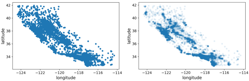
Fig. 61 . A scatter plot with full opacity (left) and alpha=0.1 (right). The transparency brings out the areas of high data density.
Images: Aurélien Géron, Hands-On Machine Learning with Scikit-Learn, Keras, and TensorFlow, Second Edition#
However it does not tell you which points are signal and which are background samples. Overall, the DataFrame plot() is a quick way to examine your data samples.
For more specific plots relevant to your optimization goals, you may have to write your own plotting macro. The reigning library for plotting in python is Matplotlib. We have started to use it in previous examples and will continue to use it in neural network training and evaluation. More will be covered during the tutorials.
Another library that is extremely convenient to get a quick glimpse at the data is seaborn. In very few lines of code, this library generates very esthetically pleasing plots. Let’s see how it looks with Scikit-Learn’s own penguin dataset:
import seaborn as sns
sns.set_theme() # apply the default theme

penguins = sns.load_dataset("penguins")
sns.jointplot(data=penguins, x="flipper_length_mm", y="bill_length_mm", hue="species")
The hue argument will produce as many series (seaborn will colour them automatically) specified.
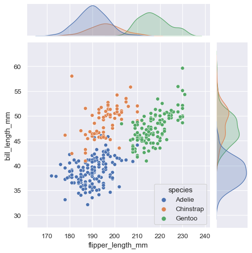
Fig. 62 . The jointplot() method in Seaborn.
Source: seaborn.pydata.org#
Another method to explore some input featuresis the pairplot(), which will draw what is called a “scatter matrix”:
sns.pairplot(data=penguins, hue="species")
It looks magnificent:
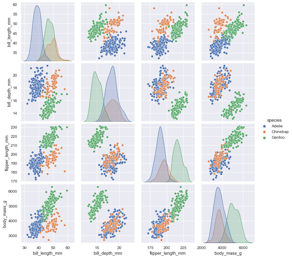
Fig. 63 . The pairplot() method in Seaborn.
Source: seaborn.pydata.org#
If you have lots of input features, you will have to select some so as to not overload the figure. Don’t forget the column storing the targets!
columns_sel = ['flipper_length_mm','bill_length_mm', 'species']
sns.pairplot(data=penguins.loc[:, columns_sel], hue="species")
Step 3. Prepare the Data#
Data Cleaning
Definition 73
Data cleaning, also called data cleansing or data scrubbing, is the process of removing incorrect, duplicate, corrupted or incomplete data within a dataset.
The visualization step before would have helped you identify possible outliers (data points with values significantly away from the rest of the data). Should they be removed? Caution! It all depends on your situation. We will see in later lectures that outliers could actually be the signal (in anomaly detection for instance). The removal of outlier should be done after gathering sufficient strong arguments about their incorrectness.
The data cleaning includes a check for duplicates, wrong or incoherent formatting, e.g. if a label is present with different spelling for instance). And also missing data. If there is a NaN (not a number) in a particular row and column, a decision should be made as most of algorithms will generate an error. A possibility is to drop the entire row, but there will be information lost on the other input features. Another way would consist of replacing the NaN with a safe value after inspecting the associated input feature.
Splitting the Datasets
As seen in Lecture 3, the data is split in three sets: training, validation and test. It can be coded manually with a cut on row indices, but one should make sure the entire dataset is shuffled before to get relatively equal representation of each class in each set. Scikit-Learn has a convenient tool to split data between a training and a testing set: the train_test_split function. To make sure the same test set is generated once the program is run again, the random_state argument ensures reproducibility:
import pandas as pd
import numpy as np
from sklearn.model_selection import train_test_split

# Not shown: X and y contains input features and targets respectively

train_set, test_set = train_test_split(X, y, test_size=0.2, random_state=42)
Feature Scaling
As seen in Lecture 2, it is recommended to scale features to prevent the gradient descent from zig-zaging along slopes differing drastically depending on the direction. This can be done manually (always a good training). Scikit-Learn has methods such as MinMaxScaler and StandardScaler.
Exercise
On which dataset(s) the feature scaling should be applied?
The training, the validation, and/or the test set(s)?
Step 4. Define the Model#
Here is the fun part of building the neural network, layers by layers (like a layered dessert).
In the model definition, there will be constraints in the input and output layers imposed by the given problem to solve:
the first layer should have as many nodes as input features
the output layer should have as many nodes as the number of expected predictions
For a regression problem, the output layer is one node dotted with a linear activation unit.
For binary classification, the output layer also has one node, but the activation function is the sigmoid.
For multi-class classification problems: the output configuration of the final layer has one node for each class, using the softmax activation function.
Example in Keras
This is real code! “DL1” is a Deep Learning algorithm developed for the ATLAS Experiment at CERN Large Hadron Collider. Elementary particles called quarks are never seen directly in the detector, they produce a spray of visible other particles called a ‘jet.’ The jet-tagging is an algorithm determining, from a jet input features, which quark type produced it: either the bottom (\(b\)), charm (\(c\)) or lighter quarks (\(s\), \(u\), \(d\)).
The model is a deep network defined this way:
from keras.layers import BatchNormalization
from keras.layers import Dense, Activation, Input, add
from keras.models import Model

# Input layer
inputs = Input(shape=(X_train.shape[1],))   #

# Hidden layers
l_units = [72, 57, 60, 48, 36, 24, 12, 6]   # nunber of nodes in each hidden layer
x = inputs
# loop to initialise the hidden layers
for unit in l_units:
    x = Dense(units=unit, activation="linear", kernel_initializer='glorot_uniform')(x)
    x = BatchNormalization()(x)
    x = Activation('relu')(x)

# Output layer
# Using softmax which will return a probability for each jet to be either light, c- or b-jet
predictions = Dense(units=3,
                    activation='softmax',
                    kernel_initializer='glorot_uniform')(x)

model = Model(inputs=inputs, outputs=predictions)
model.summary()
Credit: Manuel Guth
The input layer contains the feature (recall that .shape[1] returns the number of columns, i.e. features). The l_units list was obtained by trials and errors. ‘Dense’ for the hidden layers means the regular deeply connected neural network layer. Their non-linear activation function is ReLU. The output layer contains 3 nodes as there are 3 classes: \(b\)-jets, \(c\)-jets and light-jets. The weight initialization is done via the Glorot-Uniform, as we saw in the Section Xavier Weight Initialization.
Example in PyTorch
PyTorch is less intuitive than Keras but working at a lower level (that is to say the user has to do more coding, e.g. wrapping the methods into a loop, etc). Yet it is beneficial in terms of learning experience, as well of flexibility once the model is more complex.
Let’s see how to define a fully-connected model in PyTorch. For this we create an instance of the PyTorch base class torch.nn.Module. The __init__() method defines the layers and other components of a model, and the forward() method where the computation gets done.
Note: only the first, fourth and last hidden layers of the code above are written for conciseness.
import torch

class my_model(torch.nn.Module):

    def __init__(self, n_inputs, n_outputs):

        super(my_model, self).__init__()

        # Hidden layers:
        self.hidden1 = torch.nn.Linear(n_inputs, 72)
        self.activ1  = torch.nn.ReLU()
        self.hidden2 = torch.nn.Linear(72, 48)
        self.activ2  = torch.nn.ReLU()
        self.hidden3 = torch.nn.Linear(48, 6)
        self.activ3  = torch.nn.ReLU()
        self.hidden4 = torch.nn.Linear(6, n_outputs)
        self.activ4  = torch.nn.Softmax()

    # forward propagate input
    def forward(self, x):
        # input to first hidden layer
        X = self.hidden1(X)
        X = self.activ1(X)
        # second hidden layer
        X = self.hidden2(X)
        X = self.activ2(X)
        # third hidden layer
        X = self.hidden3(X)
        X = self.activ3(X)
        # fourth hidden layer and output
        X = self.hidden4(X)
        X = self.activ4(X)
        return X

# [...]

# Instanciation
my_model = my_model(44, 3)
The Glorot initalization can be done with the method torch.nn.init.xavier_uniform_(tensor, gain=1.0).
The gain is provided by nn.init.calculate_gain('relu'), here for the ReLU function. It needs to be inputted as gains are specific of the activation functions. More on PyTorch nn.init page.
Step 5. Train the Model#
Once we have a model, we need two things to train it: a loss function and an optimization algorithm.
Loss function
PyTorch torch.nn package has predefined loss functions. The most common ones being
MSELoss: Mean squared loss for regression.BCELoss: Binary cross-entropy loss for binary classification.CrossEntropyLoss: Categorical cross-entropy loss for multi-class classification.
Optimization algorithm
PyTorch has optimizers of the shelf thanks to its torch.optim package. Among the plethora of optimizers, some such as optim.SGD or optim.Adam should sound familiar to you. Find more on PyTorch optim page.
Let’s put things together. The train variable is a PyTorch tensor from a Dataset instance.
import torch
import torch.nn as nn

# Prepare data loaders
train_dl = DataLoader(train, batch_size=32, shuffle=True)

# [...] definition of the model my_model (above)

# Set the loss and optimization
criterion = nn.CrossEntropyLoss()
optimizer = optim.SGD(my_model.parameters(), lr=0.01, momentum=0.9)

N_epochs = 1000

# enumerate epochs
for epoch in range(N_epochs):

    # enumerate mini batches
    for i, (inputs, targets) in enumerate(train_dl):

        optimizer.zero_grad()    # clear the gradients
        yhat = my_model(inputs)  # compute the model output
        loss = criterion(yhat, targets) # calculate loss
        loss.backward()          # compute gradients
        optimizer.step()         # update model weights
It is usually more convenient to wrap this inside a user-defined function with the model and other relevant parameters as arguments. This function can then be called several times with different models.
Step 6. Tune the Model#
We saw the GridSearchCV and RandomSearchCV tools from Scikit-Learn. For neural networks, a popular library is RayTune (link to official website), which integrates with numerous machine learning frameworks. A good illustrative example is provided in Ray’s official documentation.
Step 7. Evaluate the Model#
As we saw in Step 0, the evaluation will be dictacted by the specifics of the optimization problem. It should be performed on the test set, untouched during the training. The little trick here is to ‘unconvert’ PyTorch tensors into NumPy arrays before calling the method that computes the performance metrics. A minimal implementation of a binary classifier using the accuracy would look like this:
from torch.utils.data import Dataset
from torch.utils.data import DataLoader
from numpy import vstack
from sklearn.metrics import accuracy_score

all_preds, all_obss = list(), list()

# Loop over batches
for i, (inputs, targets) in enumerate(test_dl):

    # Evaluate batch on test set
    preds = model(inputs)

    # Convert to numpy arrays
    preds = preds.detach().numpy()
    obss  = targets.numpy()
    obss  = obss.reshape((len(obss), 1))

    # Store
    all_preds.append(preds)
    all_obss.append(obss)

all_preds, all_obss = vstack(all_preds), vstack(all_preds)
# calculate accuracy
acc = accuracy_score(all_yobss, all_ypreds)
From the list of all observations all_obss and their associated predictions all_preds, it is possible to plot ROC curves and compare different models.
Step 8. Make Predictions#
Now it is time to use the model to make a prediction!
The input will be a data row of input features (but no target). A first step for PyTorch is to convert this data row into a Tensor. If row is a list:
# Convert row to data
row = torch.Tensor([row])

# Make prediction
ypred = model(row)

# retrieve numpy array
ypred = ypred.detach().numpy()

print('Predicted: %.3f (class: %d)' % (ypred, round(ypred)))
Summary: Practice Practice Practice#
You reached the end of this long page. Good. You now know the steps and building coding blocks to start your deep learning journey. But most important is practice. This will be done during tutorials and assignments. A great way to learn is to join ML competition websites such as Kaggle.com (website). Another opportunity to become better: your own project! If you are curious about a given scientific field and can find a dataset, play around driven by your own questions!
Learn More
Visualization
Matplotlib
Introduction to Seaborn
ML Framework Comparison
Tensorflow, PyTorch or Keras for Deep Learning on dominodatalab.com
PyTorch
Introduction to PyTorch Tensors - official documentation
“PyTorch Tutorial: How to Develop Deep Learning Models with Python” on machinelearningmastery.com.
Datasets & DataLoader - official documentation
TensorFlow
Official Website
TensorFlow Playground!