Stochastic Gradient Descent

Introduced in the previous lectures, Gradient Descent is a powerful algorithm to find the minimum of a function. Yet it has limitations, which are circumvented by alternative approaches, the most popular one being Stochastic Gradient Descent.

Limitations of Batch Gradient Descent

The Gradient Descent algorithm computes the cost and its derivatives using all training instances within a batch. We refer to this as Batch Gradient Descent.

Definition 66

The batch size refers to the number of training examples utilized for calculating the gradient at each iteration (epoch).

In Batch Gradient Descent, the entire training dataset is used at each step.

A convex function has a unique minimum. If the cost function is more complex, it can exhibits several minima.

There are two major drawbacks here:

• The algorithm is very slow when the training set is large

• Depending on the initial parameter values, the Gradient Descent can converge to a local minimum instead of the global minimum

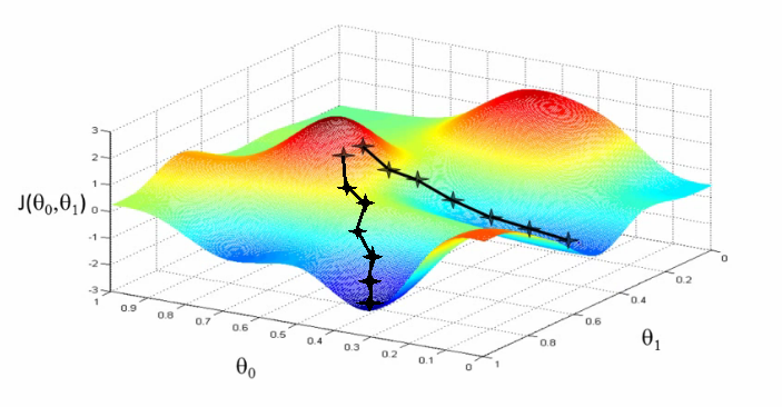
Fig. 56 . 3D representation of a cost function (height) with respect to the \(\theta\) parameters with two gradient descent paths, one towards a local minimum (right) and the other towards the global minimum (left).
_{Source: Stanford Lecture Collection}

Depending on the initial values for the \(\theta\) parameters, the gradient descent (black line) can converge to a local minimum and the associated \(\theta\) parameters will not be the most optimal ones.

Stochastic?

This term is important, let’s define it properly. It is mostly used as an adjective. Etymologically, “stochastic” comes from Greek for “guess” or “conjecture.”

Definition 67

Stochastic describes a modelling approach, or modeling techniques, involving the use of one or more random variables and probability distributions.

Stochastic is the opposite to deterministic. In determinisstic models, randomness is absent.

In some of the literature, it is said that stochastic and randomness are synonymous. There is however a difference. Randomness is used to characterize a phenomenon; nuclear decays of atom or quantum state tran are examples from nature. Stochastic refers to the modeling approach.

Actually, it is possible to apply stochastic modeling to a non-random phenomenon. For instance one can use a Monte Carlo method to approximate the value of \(\pi\).

Stochastic Gradient Descent Definition

Definition 68

Stochastic Gradient Descent is an optimization technique that performs Gradient Descent using one randomly picked training sample from the dataset.

Warning

Stochastic Gradient Descent is very sensitive to feature scaling; it is important to properly scale the feature to avoid having a stretched cost function. That would make the learning rate too small in one direction and - more problematic - too big in another direction (see Lecture 2 Section Feature Scaling & Normalization).

Important

Stochastic Gradient Descent demands the training instances to be independent and identically distributed (IID). If a datafile has one feature in ascending or descending values, the algorithm may ‘miss out’ the global minimum. To ensure that training instances are picked randomly, it is important to shuffle the training set.

Pros

• The obvious advantage of Stochastic Gradient Descent (SGD) is that it is considerably faster as there is very little data to manipulate at each epoch compared to summing over the entire dataset with Batch Gradient Descent.

• When the cost function is not convex, the SGD has a better chance to jump out of local minima.

Cons
This approach is not without drawbacks.

• The algorithm is much less smooth due to its random nature. The path (ensemble of intermediate parameter values) towards the minimum will be zigzaggy. As a consequence the cost function may go up at times; it should however decrease on average.

• The same ‘bumpy’ nature of Stochastic Gradient Descent will, once approaching the minimum, bounce around it. Therefore after the algorithm ends, the final parameter values will be closed to the optimal ones so good enough, but not the ones corresponding to the minimum.

As you see from the pros and cons above, there is a dilemma by voluntary adding randomness in the algorithm. On the one hand, it can escape local minima, i.e. getting parameter values not minimizing the cost function. But on the other hand, it never converges precisely to the optimal parameter values.

Improving Stochastic Gradient Descent

There are solutions to help the algorithm settle at the global minimum.

One of them is a compromise between Batch and Stochastic Gradient Descent called Mini-Batch Gradient Descent. Instead of picking only one training instance, a small subset of examples from the dataset are used to compute the cost derivatives. This offers a good middle ground: it is still much faster and less memory intensive than Batch Gradient Descent, will zigzag less and get closer to the read minimum than with the fully stochastic method. However the reduced noise (by summing over more samples) presents a higher risk to get stuck into a local minimum.

The other solution involves changing the learning rate \(\boldsymbol{\alpha}\), which will be covered in the next section.

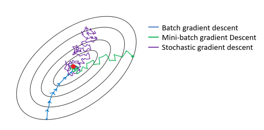
Fig. 57 . The difference in the trajectories of parameters between Batch, Mini-Batch and Stochastic Gradient Descents.
_{Image: Medium}

Exercise

Write the Stochastic Gradient Descent in pseudocode.

For reference (and inspiration), you can go back to the Gradient Descent algorithm from Lecture 2.

As we saw earlier how many computations there are in the feedforward and backpropagation algorithms in neural networks, the Stochastic Gradient Descent is the most common and popular algorithm used for training neural networks.

Learn More

Stochastic Gradient Descent on Scikit-Learn