Gradient Descent in practice

How to choose a correct learning rate?

Short answer: inspect your gradient descent cost function.

Long answer:

Adjusting the learning rate

It is always a good programming practice to add in your code printouts, i.e. print() statements to inspect the current values of your variables. In gradient descent, it is advised to print the values of the parameters and the cost function after some iterations. Here is an example of printouts of simple linear regression showing the values of updated parameters \(\theta\) every 10 epochs until \(N\) = 100, then every 100 epochs:

Starting gradient descent

Iteration 10		theta_0 = 23.360	Diff = -0.2486		theta_1 = 1.158		Diff = -0.5069		Cost = 34.1274
Iteration 20		theta_0 = 21.784	Diff = -0.1703		theta_1 = 1.590		Diff = -0.0918		Cost = 27.7958
Iteration 30		theta_0 = 20.339	Diff = -0.1423		theta_1 = 1.847		Diff = -0.0041		Cost = 23.4581
Iteration 40		theta_0 = 19.028	Diff = -0.1262		theta_1 = 2.052		Diff = 0.0133		Cost = 19.9476
Iteration 50		theta_0 = 17.841	Diff = -0.1136		theta_1 = 2.230		Diff = 0.0157		Cost = 17.0769
Iteration 60		theta_0 = 16.767	Diff = -0.1027		theta_1 = 2.390		Diff = 0.0150		Cost = 14.7278
Iteration 70		theta_0 = 15.795	Diff = -0.0929		theta_1 = 2.535		Diff = 0.0138		Cost = 12.8055
Iteration 80		theta_0 = 14.916	Diff = -0.0840		theta_1 = 2.666		Diff = 0.0125		Cost = 11.2325
Iteration 90		theta_0 = 14.121	Diff = -0.0760		theta_1 = 2.784		Diff = 0.0113		Cost = 9.9453
Iteration 200		theta_0 =  9.083	Diff = -0.0252		theta_1 = 3.534		Diff = 0.0038		Cost = 4.7867
Iteration 300		theta_0 =  7.499	Diff = -0.0093		theta_1 = 3.770		Diff = 0.0014		Cost = 4.2340
Iteration 400		theta_0 =  6.917	Diff = -0.0034		theta_1 = 3.856		Diff = 0.0005		Cost = 4.1596
Iteration 500		theta_0 =  6.704	Diff = -0.0012		theta_1 = 3.888		Diff = 0.0002		Cost = 4.1496
Iteration 600		theta_0 =  6.626	Diff = -0.0005		theta_1 = 3.900		Diff = 0.0001		Cost = 4.1483
Iteration 700		theta_0 =  6.597	Diff = -0.0002		theta_1 = 3.904		Diff = 0.0000		Cost = 4.1481
Iteration 800		theta_0 =  6.587	Diff = -0.0001		theta_1 = 3.905		Diff = 0.0000		Cost = 4.1481
Iteration 900		theta_0 =  6.583	Diff = -0.0000		theta_1 = 3.906		Diff = 0.0000		Cost = 4.1480
Iteration 1000		theta_0 =  6.581	Diff = -0.0000		theta_1 = 3.906		Diff = 0.0000		Cost = 4.1480

End of gradient descent after 1000 iterations

Picking a learning rate is a guess’n’check business.

Typical learning rates are between \(1\) and \(10^{-7}\). The common practice is to start with e.g. \(\alpha = 0.01\), a reasonable number of epochs, e.g. \(N = 100\) or \(1000\) (depending on the size of the data set), and see how the gradient descent behaves.

The cost function should decrease after every iteration. If the printouts show that the cost function and parameter are taking very, very large values: \(\alpha\) is too big, the gradient descent is diverging! One should reduce the learning rate by e.g. a factor 10 and see how the gradient behaves.

If the cost decreases after each iteration, this is a good sign that the gradient will converge. However it can converge very slowly if \(\alpha\) is too small, and as a consequence necessitate a large number of epoch before reaching the optimized parameter values. While tuning the hyperparameters, it is generally good to cap the number of epochs low and inspect the difference \(\Delta \theta = \theta^\text{new} - \theta^\text{prev}\) to see if the relative increment or decrement with respect to the \(\theta\) value is small. There is a bit of tweaking before finding a correct learning rate.

A graph to visualize the cost’s evolution

To inspect the gradient descent algorithm, it is convenient to store the intermediary values of the cost function and plot them with the iteration number on the \(x\) axis. The resulting curve should be strictly decreasing. Below is an example with different learning rates being plotted:

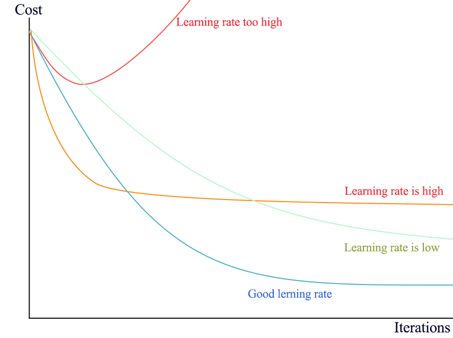
Fig. 17 . The learning rate plays a crucial role on the gradient’s speed towards convergence.
_{Credits: Jonathan Hui Medium}

Exercise

For each learning rate situation above, illustrate with a plot (qualitative drawing) the corresponding evolution of \(\theta\) parameters.

Knowing when to stop

In mathematics, zero is exactly zero. In computing, variables can store very small numbers considered zero but with trailing non-zero digits. A good cutoff to declare the gradient descent algorithm successful is to exit when e.g. the cost function’s relative decrease is lower than a given threshold, for instance \(10^{-6}\).

Summary

Linear Regression is the procedure that estimate a real-valued dependent variable (target) from independent variables (input features) assuming a linear relationship between \(n\) input features and \(n+1\) coefficients (parameters, or weight). The extra one is the offset parameter.

The cost function computes the sum of errors between the predicted line and the data. It usually uses the least squared method (errors squared).

The Gradient Descent is an optimization algorithm consisting of an iterative procedure to update the parameters in the direction of ‘descending gradient’, i.e. dictated by the slope of the cost function’s partial derivatives for each parameter, until convergence to values for the parameters minimizing the cost function.

Hyperparameters are quantitative entities controlling the learning algorithm.

The learning rate for gradient descent is an important hyperparameter that should be tuned to avoid divergence or over-shooting (learning rate too large) or slow convergence (learning rate too small) necessitating a high number of iterations (epochs).

The linear regression was our starting model. Later in this course, we will see more complex machine learning algorithms able to model non-linear behaviour. Linearity is an assumption that should be made with care.

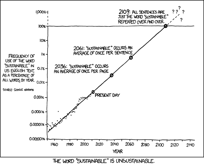
Fig. 18 . A questionable linear extrapolation, from the great webcomic xkcd.