Multivariate linear regression
Contents
Multivariate linear regression#
In machine learning, data samples contain multiple features.
We will generalize our previous definitions of linear regression to additional features. How to see this? Previously our data consisted of one column vector \(\boldsymbol{x}\) and its associated column vector of targets \(\boldsymbol{y}\). Additional input features can be visualized in the form of a table:
| x1 | x2 | x3 | x4 | |
|---|---|---|---|---|
| 0 | 49.575122 | -2.856042 | 1883.352588 | -0.019595 |
| 1 | 58.507693 | 0.793258 | 1884.420114 | -0.106611 |
| 2 | 51.854943 | 0.832562 | 2057.986212 | -0.027004 |
| 3 | 42.866146 | -2.064526 | 2028.814853 | 0.154438 |
| 4 | 54.721042 | 1.373427 | 1926.385720 | -0.093818 |
| 5 | 40.868026 | 0.279444 | 1895.182704 | -0.027091 |
The data set can be represented as a 2D array with training examples listed as rows. Here each training example has four input features \(x_1\), \(x_2\), \(x_3\) and \(x_4\). Each column lists a given feature.
In particle physics, input features can be the properties of the particles in a collision event. For instance \(x_1\) could be the electron momentum, \(x_2\) the electron’s azimutal angle of its direction in the detector’s coordinate system, \(x_3\) could be another particle’s momentum, \(x_4\) could be a special angle between two particles.
Again let’s have consistent notations:
Terminology and Notation
The number of training examples is denoted with \(m\)
The number of features is denoted with \(n\)
The row index or rank of a training example is in superscript, from 1 to \(m\)
The feature or column of a training example is in subscript, from 1 to \(n\)
\(\Rightarrow\) the value of input feature \(j\) of training example in row \(i\) is
The training examples form a (\(m \times n\)) matrix \(X\):
Warning
The \(i^\text{th}\) training sample \(\boldsymbol{x^{(i)}}\) is not a scalar but a row vector of \(n\) elements.
Our hypothesis function is generalized to the following for a given training example (row \(i\)):
Definition 9
The hypothesis or mapping function for linear regression with \(n\) features is:
Warning
There are \(n+1\) parameters to optimize as we need to add the offset parameter \(\theta_0\).
If we set \(x_0^{(i)} = 1\), we can write the mapping function as a sum. For one training example \(x^{(i)}\), i.e. a row in the data set:
where \(x^{(i)}\) an row vector of \(n+1\) elements, \(x^{(i)} = (x^{(i)}_0, x^{(i)}_1, x^{(i)}_2, \cdots, x^{(i)}_n)\) and \(\theta\) is a row vector too of \(n+1\) elements as well, \(\theta = (\theta_0, \theta_1, \cdots, \theta_n)\). Thus taking the transposed is equivalent to a dot product:
Gradient Descent in Multilinear Regression#
We will revisit our algorithm to generalize it to \(\theta_n\) parameters:
Algorithm 2 (Gradient Descent for Multivariate Linear Regression)
Inputs
Training data set \(X\) of \(m\) samples with each \(n\) input features, associated with their targets \(y\):
Hyperparameters
Learning rate \(\alpha\)
Number of epochs \(N\)
Outputs
The optimized values of \(\theta\) parameters, \(\theta_0\), \(\theta_1\), … , \(\theta_n\) minimizing \(J(\theta)\).
Initialization: Set values for all \(\theta\) parameters
Iterate N times or while the exit condition is not met:
Derivatives of the cost function:
Compute the partial derivatives \(\frac{\partial }{\partial \theta_j} J(\theta)\) for each \(\theta_j\)Update the parameters:
Calculate the new parameters according to:
(8)#\[\begin{split}\begin{equation*} \\ \theta'_j = \theta_j-\alpha \frac{\partial}{\partial \theta_j} J\left(\theta\right) \; \; \; \; \; \; \forall j \in [0..n]\\ \end{equation*}\end{split}\]Reassign the new \(\theta\) parameters to prepare for next iteration
Exit conditions
After the maximum number of epochs \(N\) is reached
If all derivatives are zero:
The partial derivatives of \(J(\theta)\) for each parameter \(\theta_j\) will be of the form:
Feature Scaling & Normalization#
In the example of the previous section, the 3D plot of the cost function with respect to the \(\theta\) parameters was not really bowl-shaped but stretched. This happens when the features are of different ranges. One parameter will have an increment size larger than the other.
Exercise
If let’s say \(x_1\) has values between \(10 000\) and \(100000\) and \(x_2\) between 1 and 10.
Which parameter, \(\theta_1\) or \(\theta_2\) will be updated with a very large or very small step? (independently of the sign). Hint: ask yourself in which direction the contour is going to be stretched.
What are the consequences on the gradient descent algorithm?
Check your answers
Answer 1. If \(x_1\) contains very large values, the coefficients \(\theta_1\) will have to be very small and tuned in a fine way to not let the cost function explode. The \(\theta_2\) parameters will not have to be tuned that finely to prevent the cost function from getting big. Thus the contour plot will be stretched along the parameter associated with the features spanning a small range.
The \(\theta\) parameters will descend (or converge) slowly on large ranges and quickly on small ranges, as the figure below shows:
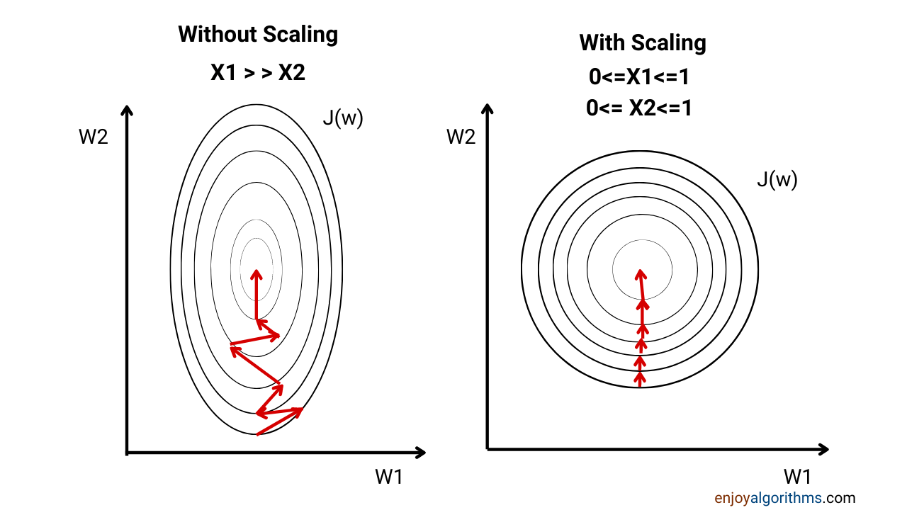
Fig. 14 . The contour without feature scaling is skewed and takes up an oval shape. If normalized, the path towards the minimum is shorter.
Source: enjoyalgorithms.com #
Answer 2. The difference in range can lead to an ‘overshooting’ of one parameter value to the other side of the slope, thus creating a zig-zag path towards the minimum. It will slow down the learning process, because more steps are needed before converging to the minimum of the cost function. Another consequence is the risk of divergence: as the learning rate \(\alpha\) is the same while updating all parameters, a big jump in one direction can even lead to instability (more on that in the next section).
What is feature scaling?#
Definition 10
Feature scaling is a data preparation process consisting of harmonizing the values of the input variables taken as features for a machine learning algorithm.
Feature scaling can be implemented in different ways. We will see the two classics: mean normalization and standardization.
Mean normalization#
Definition 11
Mean normalization consists of calculating the mean \(\mu_j\) of all training examples \(x_j^{(1)}, x_j^{(2)}, \cdots, x_j^{(m)}\) of a given feature \(j\) and subtract it to each example \(x_j^{(i)}\) of that feature:
It is usual to divide by the range of the features:
Consequence: the mean of the new normalized sample collection for that feature - think of it as an extra column in the matrix \(X\) - will be zero. The data distribute the same as before, the values are just representing the distance to the mean.
Standardization#
Definition 12
Standardization is a mean normalization procedure using as denominator the standard deviation \(\sigma_j\) of all the samples for a given feature.
Consequence: the mean and standard deviation of the new normalized collection of feature \(j\) will be zero and one respectively.
When is feature scaling relevant? When is it not?
It all depends on how the data look like. This is why it is important before starting the machinery of (fancy) learning techniques to inspect the data, plot several distributions if possible and dedicate time for the preparedness steps: data cleaning, scaling etc. This is essential for the success of the fitting algorithm.