Cost Function for Classification
Contents
Cost Function for Classification#
Wavy least squares#
If we plug our sigmoid hypothesis function \(h_\theta(x)\) into the cost function defined for linear regression (Equation (3) from Lecture 2), we will have a complex non-linear function that could be non-convex. The cost function could take this form:
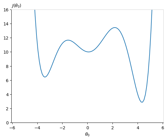
Imagine running gradient descent starting from a randomly initialized \(\theta_0\) parameter around zero (or worse, lower than -2). It will fall into a local minima. Our cost function will not be at the global minimum! It is crucial to work with a cost function accepting one unique minimum.
Building a new cost function#
As we saw in the previous section, the sigmoid fits the 1D data distribution very well. Our cost function will use the hypothesis \(h_\theta(x)\) function as input. Recall that the hypothesis \(h_\theta(x)\) is bounded between 0 and 1. What we need is a cost function producing high values if we mis-classify events and values close to zero if we correctly label the data. Let’s examine what we want for the two cases:
Case of a signal event:
A data point labelled signal verifies by our convention \(y=1\). If our hypothesis \(h_\theta(x)\) is also 1, then we have a good prediction. The cost value should be zero. If however our signal sample has a wrong prediction \(h_\theta(x) = 0\), then the cost function should take large values to penalize this bad prediction. We need thus a strictly decreasing function, starting with high values and cancelling at the coordinate (1, 0).
Case of a background event:
The sigmoid can be interpreted as a probability for a sample being signal or not (but note it is not a probability distribution function). As we have only two outcomes, the probability for a data point to be non signal will be in the form of \(1 - h_\theta(x)\). We want to find a function with this time a zero cost if the prediction \(h_\theta(x) = 0\) and a high cost for an erroneous prediction \(h_\theta(x) = 1\).
Now let’s have a look at these two functions:
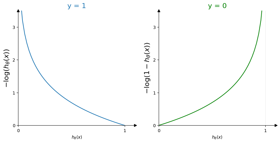
For each case, the cost function has only one minimum and harshly penalizes wrong prediction by blowing up at infinity.
How to combine these two into one cost function for logistic regression?
Like this:
Definition 19
The cost function for logistic regression is defined as:
This function is also called cross-entropy loss function and is the standard cost function for binary classifiers.
Note the negative sign factorized at the beginning of the equation. The first and second term inside the sum are multiplied by \({\color{RoyalBlue}y^{(i)}}\) and \({\color{OliveGreen}(1 - y^{(i)})}\). This acts as a “switch” between the two possible cases for the targets: \({\color{RoyalBlue}y=1}\) and \({\color{OliveGreen}y=0}\). If \({\color{RoyalBlue}y=1}\), the second term cancels out and the cost takes the value of the first. If \({\color{OliveGreen}y=0}\), the first term vanishes. The two mutually exclusive cases are combined into one mathematical expression.
Gradient descent#
The gradient descent for classification follows the same procedure as described in Algorithm 2 in Section Gradient Descent in Multilinear Regression with the definition of the cost function from Equation (13) above.
Derivatives in the linear case#
Consider the linear assumption \(x^{(i)}\theta^{\; T} = \theta_0 + \theta_1 x_1 + \cdots + \theta_n x_n\) as input to the sigmoid function \(f\). The cost function derivatives will take the form:
This takes the same form as the derivatives for linear regression, see Equation (10) in Section Gradient Descent in Multilinear Regression.
Alternative techniques#
Beside logistic regression, other algorithms are designed for binary classification.
The Perceptron, which is a single layer neural network with, in its original form, a step function instead of a sigmoid function. We will cover neural networks in Lectures 6 and 7.
Support Vector Machines (SVMs) are robust and widely used in classification problems. We will not cover them here but below are some links for further reading.
Learn more
R. Berwick, An Idiot’s guide to Support vector machines (SVMs) on web.mit.edu
Support Vector Machines: A Simple Explanation, on KDNuggets
Support Vector Machines: Main Ideas” by Josh Starmer, on StatQuest YouTube channel
Numerous methods have been developed to find optimized \(\theta\) parameters in faster ways than the gradient descent. These optimizers are beyond the scope of this course and usually available as libraries within python (or other languages). Below is a list of the most popular ones:
Learn more
The BFGS algorithm: Wikipedia article
The Limited-memory BFGS, L-BFGS: Wikipedia article
Conjugate gradient method: Wikipedia article
More than two categories: multiclassification#
We treated the binary classification problem. How to adapt to a situation with more than two classes?
Let’s for instance consider three classes, labelled with their colours and distributed in two dimensions (two input features) like this:
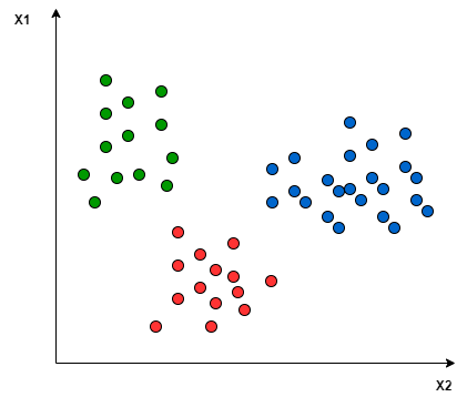
Fig. 20 . 2D distribution of three different classes.
Image: analyticsvidhya.com#
A multi-class classification problem can be split into multiple binary classification datasets and be trained as a binary classification model each. Such approach is a heuristic method, that is to say not optimal nor direct. But it eventually does the job. There are two main approaches of such methods for multiclassification.
Definition 20
The One-to-One approach consists of applying a binary classification for each pair of classes, ignoring the other classes.
With a dataset made of \(N^\text{class}\) classes, the number of models to train, \(N^\text{model}\) is given by
Each model predicts one class label. The final decision is the class label receiving the most votes, i.e. being predicted most of the time.
Pro
The sample size is more balanced between the two chosen classes than if datasets were split with one class against all others.
Con
The pairing makes the number of models to train large and thus computer intensive.
Definition 21
The One-to-All or One-to-Rest approach consists of training each class against the collection of all other classes.
With a dataset made of \(N^\text{class}\) classes, the number of pairs to train is
The final prediction is given by the highest value of the hypothesis function \(h^{k}_\theta(x)\), \(k \in [1, N^\text{model}]\) among the \(N^\text{model}\) binary classifiers.
Pro
Less binary classifiers to train.
Con
The number of data points from the class to look for will be very small if the ‘background’ class is the merging of all other data points from the other classes.
Illustrations.
The One-to-One method would create those hyperplanes (with two input features, D = 2 we will have a 1D line as separation):
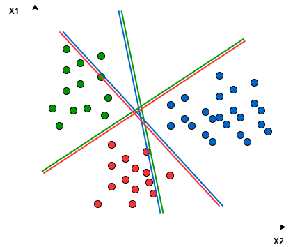
Fig. 21 . One-to-One approach splits paired datasets, ignoring the points of the other classes.
Image: analyticsvidhya.com#
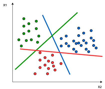
Fig. 22 . One-to-All approach focuses on one class to discriminate from all other points
(i.e. all other classes are merged into a single ‘background’ class).
Image: analyticsvidhya.com#
Some further reading if you are curious: