Logistic Regression: introduction

Before getting into the details here are some general definitions.

Definitions

Definition 13

Logistic regression is a statistical model used in machine learning to make a prediction from one or more independent variables about a categorical variable as target.

Definition 14

A categorical variable is a variable that can take a limited number of possible values.
Examples: true or false, yes or no, the 10 digits from 0 to 9, the 26 letters of the latin alphabet, etc.

In other words, logistic regression is about making predictions about a discrete variable instead of a continuous one.

Definition 15

Binary classification refers to a classification task into two mutually exclusive categories.

Multi-class classification refers to a classification task that has more than two categorical variables.

Motivations

Let’s start with a simple case with only one input variable.

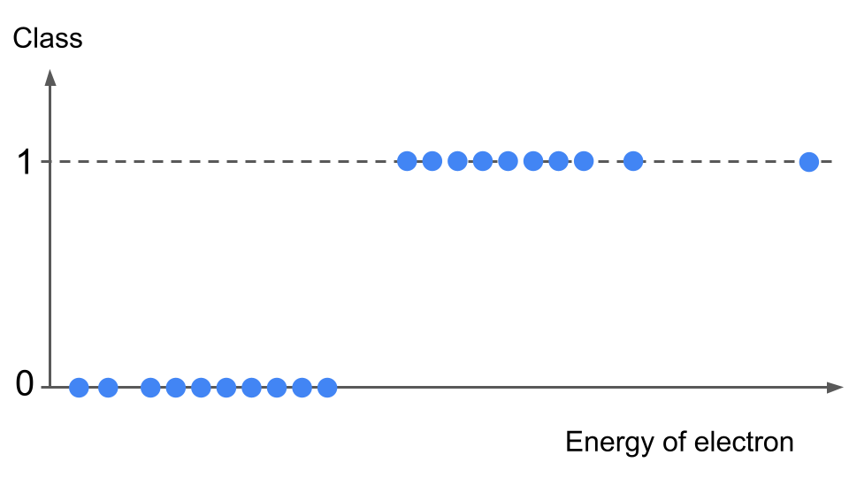
Particle detectors are usually equiped with a trigger system. It is a program assessing raw data. Its mission is to quickly decide if a given interaction event is worth saving into disk for further analysis or not. Using previous data analyzed offline (i.e. with more complex software), it is possible to gather more information on the events and objects in it (objects are reconstructed particles with all associated properties). For instance, the energy of the electron can be a good hint to help predict if the event where the electron is produced will be selected for further physics study. The workflow is a bit more complex; we will simplify and label such “selected event” as “signal event” and those that are later discarded during the data analysis “background event”. The signal events are associated with 1 and background events with 0. This is a binary classification problem.

Warning

The association of a given class to a discrete value is a arbitrary and done as a convention. In some cases 1 can stand for what we want to look for in the data (i.e. signal electron in our example above). But in other fields, medical diagnosis for instance, 1 can code for a malign tumor and 0 a benign tumor. It is very important to define the bijection of your classes and the associated values and stick to your convention while building your machine learning program.

We can visualize the data as a scatter plot like this:

If we use the linear regression method, our hypothesis function \(h(x)\) will be a line (the two examples drawn below are qualitative only):

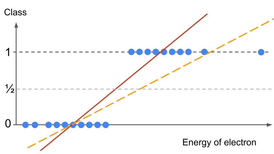
How can we predict a probability? We could use the 0.5 mark as our threshold. Given an electron energy input \(x\), if \(h(x)>0.5\) then we predict the event is a signal event, if \(h(x) < 0.5\) then the event is classified as background.

We can already see a problem: our hypothesis outputs values departing from the data labels: zero and ones. Worse, the hypothesis has values either below or above one, i.e. outside of the label range! What does the errors (going to be very large at the extremes) mean? Would the cost function really represent the global error? This is a first hint that applying linear regression is not well adapted here.

Worse: imagine we have an event with a very high energy for the electron (see the data point on the very far right of the plot above). Intuitively, this should be classified as signal from what we see above. However, a linear regression will shift the hypothesis function (orange dashed line) towards the right, in order to minimize the error from this far-right data point. Consequence? We will mis-classify several data points, correctly labelled as signal before, into the background category!

From this introduction, it is clear that linear regression is not adapted for our classification problem. This is when the sigmoid function enters the game!