Regularization

A converging gradient descent is not the end of the story. The learning algorithm can fit the data too specifically to the training samples and would fail once given additional data, compromising the accuracy of predictions: this is overfitting. To prevent this, a regularizing term is added in the cost function to constrain the parameters.

Underfitting, overfitting

Definition 22

Underfitting is a situation that occurs when a fitting procedure or machine learning algorithm is not capturing the general trend of the dataset.

Another way to put it: an underfit algorithm lacks complexity.

The antonym of underfitting is overfitting.

Definition 23

Overfitting is a situation that occurs when a fitting procedure or machine learning algorithm matches too precisely a particular collection of a dataset.

Overfitting is synonym of overtuned, overtweaked. In other words: the model learns the detail and noise in the training dataset to the extent that it negatively impacts the performance of the model on a new dataset. This means that the noise or random fluctuations in the training dataset is picked up and learned as concepts by the model. In machine learning, we look for trends and compromises: a good algorithm may not be perfectly classifying a given data set; it needs to accommodate and ignore rare outliers so that future predictions, on average, will be accurate (we will see how to diagnose learners in the next section).

The problem with overfitting is the future consequences once the machine learning algorithm receives additional data: it may lack flexibility.

Definition 24

The flexibility of a model determines its ability to generalize to different characteristic of the data.

In some definitions (it seems there is no standard definition of flexibility), the literature quotes “to increase the degrees of freedom available to the model to fit to the training data.” What are degrees of freedom in this context? Think of data points distributed along a parabola. A linear model will be underfitting the data as it is too simple to catch the parabolic trend with only two degrees of freedom (remember there are two parameters to optimize). A quadratic equation, however, will manage well with three degrees of freedom. A model with more degrees of freedom has margin to adapt well to different situations. This is the idea behind flexibility.

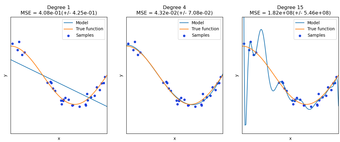
Fig. 23 . Example of several regression models.
The linear one on the left (Degree 1) is underfitting the data. The model on the right (Degree 15) is overfitting the data as its high polynomial produces a curve over-specific to the given data set. The middle model (Degree 4) is a good compromise.
_{Source: scikit-learn.org (with associated python code)}

How to avoid overfitting?

Regularization types

Definition 25

Regularization in machine learning is a processus consisting of adding constraints on a model’s parameters.

The two main types of regularization techniques are the Ridge Regularization (also known as Tikhonov regularization, albeit the latter is more general) and the Lasso Regularization.

Ridge Regression

The Ridge regression is a linear regression with an additional regularization term added to the cost function:

(17)\[ J(\theta) = \frac{1}{2m} \left[ \sum_{i=1}^{m} \left( h_\theta(x^{(i)}) - y^{(i)}\right)^2 + {\color{Maroon}\lambda \sum_{j=1}^n \theta_j^2} \right]\]

The hyperparameter \(\lambda\) controls the degree of regularization. If \(\lambda = 0\), the regularization term vanishes and we have a non-regularized linear regression. You can see the penalty imposed by the term \(\lambda\) will force the parameters \(\theta\) to be as small as possible; this helps avoiding overfitting. If \(\lambda\) gets very large, the parameters can be so shrinked that the model becomes over-simplified to a straight line and thus underfit the data.

Note

The factor \(\frac{1}{2}\) is used in some derivations of the regularization. This makes it easier to calculate the gradient, however it is only a constant value that can be compensated by the choice of the parameter \(\lambda\).

Warning

The offset parameter \(\theta_0\) is not entering in the regularization sum.

In the litterature, the parameters are denoted with \(b\) for the offset (bias) and a vector of weight \(\vec{w}\) for the other parameters \(\theta_1, \theta_2, \cdots \theta_n\). Thus the regularization term is written:

(18)\[\lambda \left(\left\| \vec{w} \right\|_2\right)^2\]

The \(\ell_2\) norm is the Euclidian norm \(\left\| x \right\|_2 = \sqrt{x_0^2 + x_1^2 + \cdots + x_n^2}\).

with \(\left\| \vec{w} \right\|_2\) the \(\ell_2\) norm of the weight vector.

For logistic regression, the regularized cost function becomes:

(19)\[ J(\theta) = - \frac{1}{m} \sum^m_{i=1} \left[ \;\; y^{(i)} \log( h_\theta(x^{(i)} )) \;+\; (1- y^{(i)}) \log( 1 - h_\theta(x^{(i)} )) \;\;\right] + {\color{Maroon}\frac{\lambda}{2m} \sum_{j=1}^n \theta_j^2}\]

Lasso Regularization

The \(\ell_1\) norm is the sum of the magnitudes of the vectors. It is also called Manhattan or Taxicab norm.

Lasso stands for least absolute shrinkage and selection operator. Behind the long acronym is a regularization of the linear regression using the \(\ell_1\) norm. We denote Cost(\(\theta\)) the cost function, i.e. either the Mean Squared Error for linear regression or the cross-entropy loss function (13) for logistic regression. The lasso regression cost function is

(20)\[J(\theta) = \text{Cost(}{\theta}\text{)} + {\color{Maroon}\frac{\lambda}{2m} \sum_{j=1}^n | \theta_j | }\]

The regularizing term uses the \(\ell_1\) norm of the weight vector: \(\left\| \vec{w} \right\|_1\).

Warning

As regularization influences the parameters, it is important to first perform feature scaling before applying the regularization.

Which regularization method to use?

Each one has its pros and cons. As \(\ell_1\) (lasso) is a sum of absolute values, it is not differentiable and thus more computationally expensive. Yet \(\ell_1\) better deals with outliers (extreme values in the data) by not squaring their values. It is said to be more robust, i.e. more resilient to outliers in a dataset.

The \(\ell_1\) regularization, by shriking some parameters to zero (making them vanish and no more influencial), has feature selection built in by design. If this can be advantageous in some cases, it can mishandle highly correlated features by arbitrarily selecting one over the others.

Additional reading are provided below to deepen your understanding in the different regularization methods. Take home message: both methods combat overfitting.

Learn more

• A comparison of the pros and cons of Ridge (\(\ell_2\) norm) and lasso (\(\ell_1\) norm) regularization: “L1 Norms versus L2 Norms”, Kaggle

• Fighting overfitting with \(\ell_1\) or \(\ell_2\) regularization, neptune.ai

How can we inspect our machine learning algorithm to assess, even quantify the presence of under or overfitting? This is what we cover in the next section.