Activation Functions

As we saw in the previous section, the nodes in hidden layers, aka the “activation units,” receive input values from data or activation units of the previous layer. Each time a weighted sum is computed. Then the activation function defines which value, by consequence importance, the node will output. Before going of the most common activation functions for neural networks, it is essential first to introduce their properties as they illustrate core concepts or neural network learning process.

Mathematical properties and consequences

Differentiability

We will see in the next lecture that the backpropagation, the algorithm adjusting all network’s weights and biases, involves a gradient descent procedure. It is thus desirable for the activation function to be continously differentiable (but not strictly necessary, as we will see soon for particular functions). The Heaviside step function of the perceptron has a derivative undefined at \(z=0\) and the gradient is zero for all \(z\) otherwise: a gradient descent procedure will not work here as it will ‘stagnate’ and never start descending as it always returns zero.

Range

The range concerns the interval of the activation function’s output values. In logistic regression, we introduced the sigmoid function mapping the entire input range \(z \in \mathbb{R}\) to the range [0,1], ideally for binary classification. Activation functions with a finite range tend to exhibit more stability in gradient descent procedures. However it can lead to issues know as Vanishing Gradients explained in the next subsection The risk of vanishing or exploding gradients.

Non-linearity

This is essential for the neural network to learn. Explanations. Let’s assume there is no activation function. Every neuron will only be performing a linear transformation on the inputs using the weights and biases. In other words, they will not do anything fancier than \((\sum wx + b)\). As the composition of two linear functions is a linear function itself (a line plus a line is a line), no matter how many nodes or layers there are, the resulting network would be equivalent to a linear regression model. The same simple output achieved by a single perceptron. Impossible for such an network to learn complex data patterns.

What if we use the trivial identify function \(f(z) = z\) on the weighted sum? Same issue: all layers of the neural network will collapse into one, the last layer will still be a linear function of the first layer. Or to put it differently: it is not possible to use gradient descent as the derivative of the identity function is a constant and has no relation to its input \(z\).

There is a powerful result stating that only a three-layer neural network (input, hidden and output) equiped with non-linear activation function can be a universal function approximator within a specific range:

Theorem 1

In the mathematical theory of artificial neural networks, the Universal Approximation Theorem states that a forward propagation network of a single hidden layer containing a finite number of neurons can approximate continuous functions on compact subsets of \(\mathbb{R}^n\).

When is meant behind “compact subsets of \(\mathbb{R}\) is that the function should not have jumps nor large gaps. This is quite a remarkable result. The simple multilayer perceptron (MLP) can thus mimick any known function, from cosine, to exponential and even more complex curves!

Main activation functions

Let’s present some common non-linear activation functions, their characteristics, with the pros and cons.

The sigmoid function

We know that one! A reminder of its definition:

\[\sigma(z) = \frac{1}{1 + e^{-z}}\]

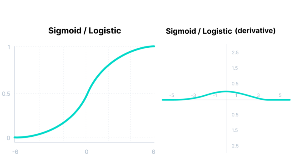
Fig. 45 . The sigmoid activation function and its derivative.
_{Image: www.v7labs.com}

Pros

• It is a very popular choice, mostly due to the output range from 0 to 1, convenient to generate probabilities as output.

• The function is differentiable and the gradient is smooth, i.e. no jumps in the ouput values.

Cons

• The sigmoid’s derivative vanishes at its extreme input values (\(z \rightarrow - \infty\) and \(z \rightarrow + \infty\)) and is thus proned to the issue called Vanishing Gradient problem (see The risk of vanishing or exploding gradients).

Hyperbolic Tangent

Alike the sigmoid, the hyperbolic tangent is S-shaped and continously differentiable. The output values range is different from the sigmoid, as it goes from -1 to 1.

(53)\[\tanh(z) = \frac{e^z - e^{-z}}{e^z + e^{-z}}\]

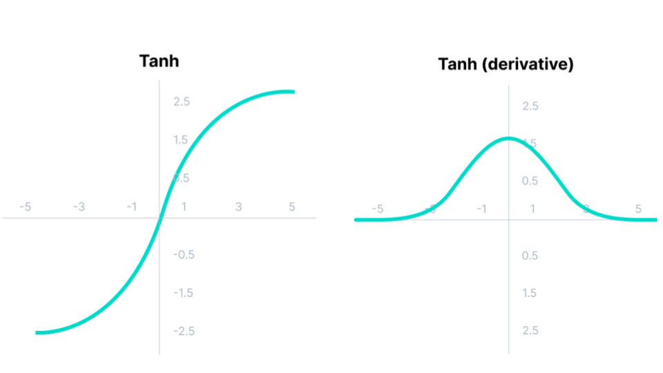
Fig. 46 . The hyperbolic tangent function and its derivative.
_{Image: www.v7labs.com}

Pros

• It is zero-centered. Unlike the sigmoid when we had to have a decision boundary of \(0.5\) (half the output range), here the mapping is more straightforward: negative input values gets negative output, and positive input values will be positive, with one point (\(z=0\)) returning a neutral output of zero.

• That fact the mean of the ouput values is close to zero (middle of the output range) makes the learning easier.

Cons

• The gradient is much steeper than for the sigmoid (risk of jumps while descending)

• There is also a Vanishing Gradient problem due to the derivative cancelling for \(z \rightarrow - \infty\) and \(z \rightarrow + \infty\).

Rectified Linear Unit (ReLU)

Welcome to the family of rectifiers, thee most popular activation function for deep neural networks. The ReLU is defined as:

(54)\[f(z) = \max(0,z)\]

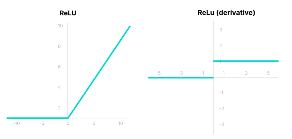
Fig. 47 . The Rectified Linear Unit (ReLU) function and its derivative.
_{Image: www.v7labs.com}

Pros

• Huge gain in computational efficiency (much faster to compute than the sigmoid or tanh)

• Only 50% of hidden activation units are activated on average (it is called sparse activation), further improving the computational speed

• Better gradient descent as the function does not saturate in both directions like the sigmoid and tanh. In other words, the Vanishing Gradient problem is half reduced

Cons

• Unlike the hyperbolic tangent, it is not zero-centered

• The range is infinite for positive input value (not bounded)

• ReLU is not differentiable at zero (but this can be solved by choosing arbitrarily a value for the derivative of either 0 or 1 for \(z=0\) )

• The “Dying ReLU problem”

What is the Dying ReLU problem? When we look at the derivative, we see the gradient on the negative side is zero. During the backpropagation algorithm, the weights and biases are not updated and the neuron becomes stuck in an inactive state. We refer to it as ‘dead neuron.’ If a large number of nodes are stuck in dead states, the model capacity to fit the data is decreased.

To solve this serious issue, rectifier variants of the ReLU have been proposed:

Leaky ReLU

It is a ReLU with a small positive slope for negative input values:

(55)\[\begin{split}\text{Leaky ReLU}(z) =\begin{cases}\;\; 0.01 z & \text{ if } z < 0 \\\;\; z & \text{ if } z \geq 0\end{cases} \;\;\;\; \forall \: z \in \mathbb{R}\end{split}\]

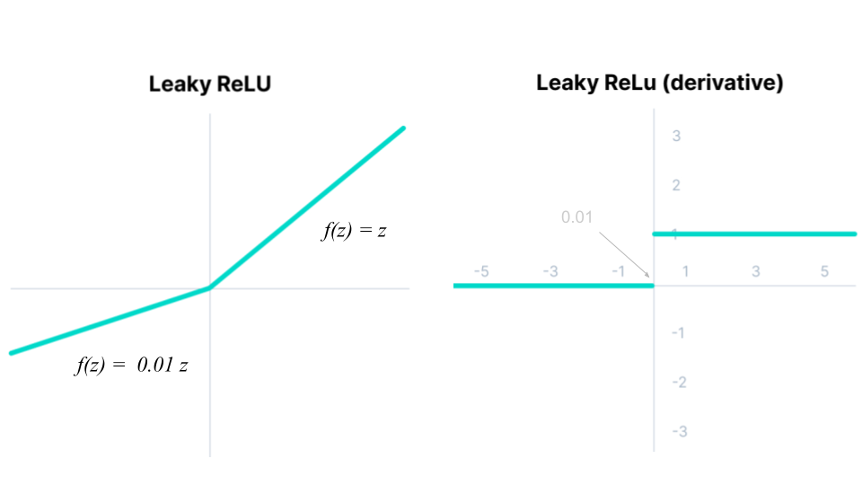
Fig. 48 . The Leaky Rectified Linear Unit (ReLU) function and its derivative. The gradient in the negative area is 0.01, not zero.
_{Image: www.v7labs.com}

The Leaky ReLU offers improvements compared to the classical ReLU:

Pros

• All advantages of the ReLU mentioned above (fast computation, no saturation for positive input values)

• The small positive gradient when units are not active makes it possible for backpropagation to work, even for negative input values

• The non-zero gradient mitigate the Dying ReLU problem

Cons

• The slope coefficient is determined before training, i.e. it is not learnt during training

• The small gradient for negative input value requires a lot of iterations during training: the learning is thus time-consuming

Parametric ReLU (PReLU)

The caveat of the Leaky ReLU is addressed by the Parametric ReLU (PReLU), where the small slope of the negative part is tuned with a parameter that is learnt during the backpropagation algorithm. Think of it as an extra hyper-parameter of the network.

(56)\[\begin{split}\text{Parametric ReLU}(z) =\begin{cases}\;\; a z & \text{ if } z < 0 \\\;\; z & \text{ if } z \geq 0\end{cases} \;\;\;\; \forall \: z, a \in \mathbb{R}, a > 0\end{split}\]

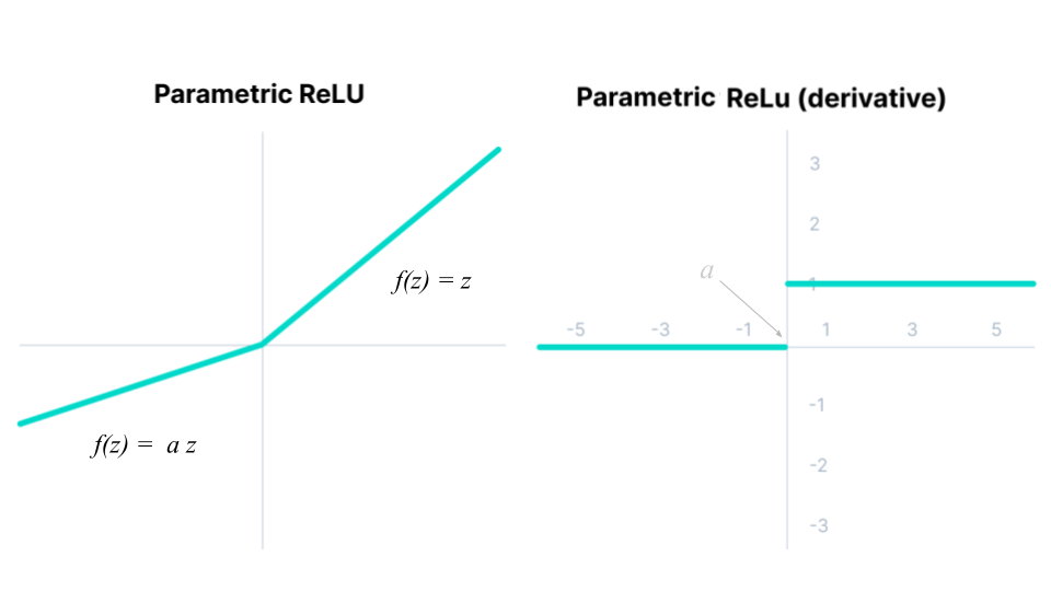
Fig. 49 . The Parametric Rectified Linear Unit (ReLU) function and its derivative.
_{Image: www.v7labs.com}

Pros

• The parametric ReLU collects all advantages of the ReLU and takes over when the Leaky ReLU still fails too reduce the number of dead neurons

Cons

• There is an extra parameter to tweak in the network, the slope value \(a\), which is not trivial to get as its optimized value is different depending on the data to fit

Exponential Linear Units (ELUs)

It does not have Rectifier in the name but the Exponential Linear Unit is another variant of ReLU.

\[\begin{split}\text{ELU}(z) =\begin{cases}\;\; a(e^z -1) & \text{ if } z < 0 \\\;\; z & \text{ if } z \geq 0\end{cases} \;\;\;\; \forall \: z , a \in \mathbb{R}, a > 0\end{split}\]

with \(a\) a hyper-parameter to be tuned.

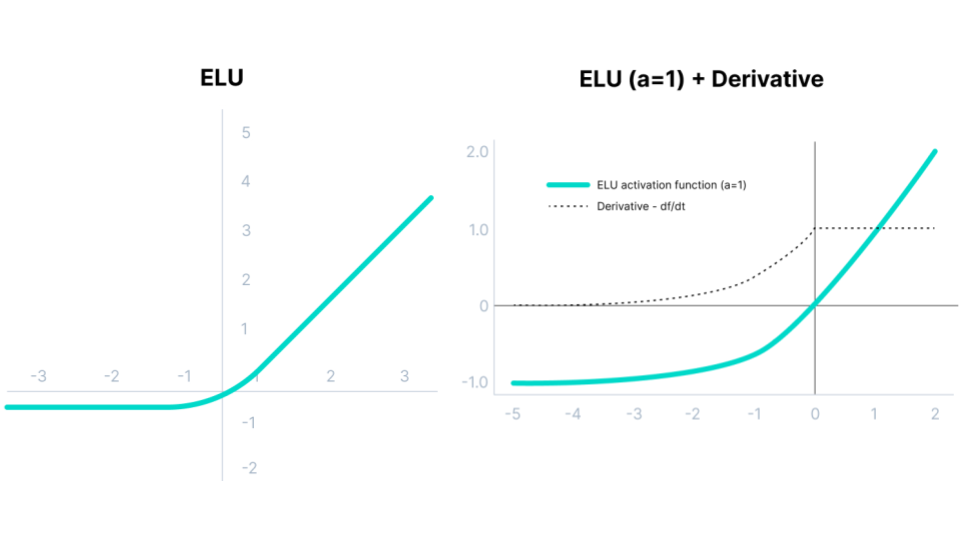
Fig. 50 . The Exponential Linear Unit (ELU) function and its derivative.
_{Image: www.v7labs.com}

Pros

• From high to low input values, the ELU smoothly decreases until it outputs the negative value \(-a\). There is no more a ‘kick’ like in ReLU

• ELU functions have shown to converge cost to zero faster and produce more accurate results

Cons

• The parameter \(a\) needs to be tuned; it is not learnt

• For positive inputs, there is a risk of experiencing the Exploding Gradient problem (explanations further below in The risk of vanishing or exploding gradients)

Scaled Exponential Linear Unit (SELU)

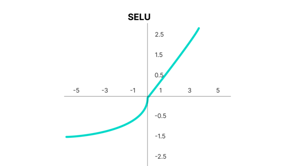
Fig. 51 . The Scaled Exponential Linear Unit (SELU) function.
_{Image: www.v7labs.com}

The Scaled Exponential Linear Unit (SELU) is defined as:

\[\begin{split}\text{ELU}(z) = \lambda \begin{cases}\;\; a(e^z -1) & \text{ if } z < 0 \\\;\; z & \text{ if } z \geq 0\end{cases} \;\;\;\; \forall \: z , a \in \mathbb{R},\end{split}\]

where \(\lambda = 1.0507\) and \(a = 1.67326\). Why these specific values? The values come from a normalization procedure; the SELU activation introduces self-normalizing properties. It takes care of internal normalization which means each layer preserves the mean and variance from the previous layers. SELU enables this normalization by adjusting the mean and variance. It can be shown that, for self-normalizing neural networks (SNNs), neuron activations are pushed towards zero mean and unit variance when propagated through the network (there are more details and technicalities in this paper for those interested).

Pros

• All the rectifier’s advantages are at play

• Thanks to internal normalization, the network converges faster

Cons

• Not really a caveat in itself, but the SELU is outperforming other activation functions only for very deep networks

Gaussian Error Linear Unit (GELU)

Another modification of ReLU is the Gaussian Error Linear Unit. It can be thought of as a smoother ReLU.
The definition is:

\[\text{GELU}\left(z\right) = z\; \Phi\left(z\right) = z \cdot \frac{1}{2}\left[1 + \text{erf}\left(\frac{z}{\sqrt{2}} \right)\right]\]

where \(\Phi(z)\) is the cumulative distribution function of the standard normal distribution.

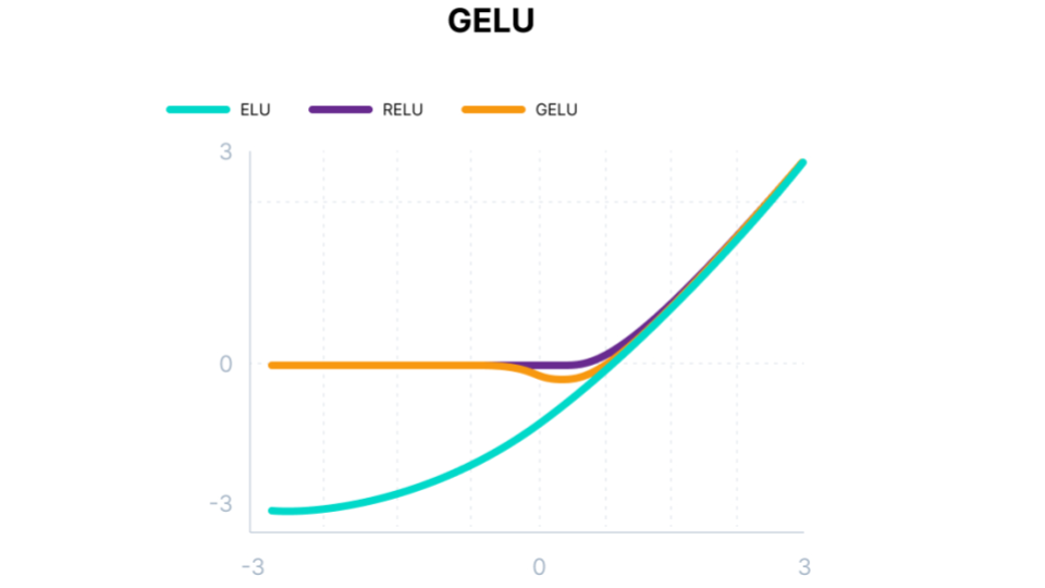
Fig. 52 . The Gaussian Error Linear Unit (GELU) function overlaid with ReLU and ELU.
_{Image: www.v7labs.com}

GELU is the state-of-the-art activation function used in particular in models called Transformers. It’s not the movie franchise; the Transformer model was introduced by Google Brain in 2017 to help in the multidisciplinary field of Natural Language Processing (NLP) that deals, among others, with tasks such as text translation or text summarization.

Pros

• Differentiable for all input values \(z\)

• Avoids the Vanishing Gradient problem

• As seen above, the function is non-convex, non-monotonic and not linear in the positive domain: it has thus curvature at all points. This actually allowed GELUs to approximate better complicated functions that ReLUs or ELUs can as it weights inputs by their value and not their sign (like ReLu and ELU do)

• The GELU, by construction, has a probabilistic interpretation (it is the expectaction of a stochastic regularizer)

Cons

• GELU is time-consuming to compute

Sigmoid Linear Unit (SiLU) and Swish

The original definition is defined as \(f(z) = x \cdot \text{sigmoid}(\beta z)\), with \(\beta\) a learnable parameter. Yet as most implementations set \(\beta =1\), the function is usually named “Swish-1”. But if \(\beta \rightarrow \infty\), then the Swish becomes like the ReLU function.

The SiLU and Swish are the same function, just introduced by different authors (the Swish authors are from Google Brain). It is a state-of-the-art function aiming at superceeding the hegemonic ReLU. The Swish is defined as a sigmoid multiplied with the identity:

\[f(z) = \frac{z}{1 + e^{-z}}\]

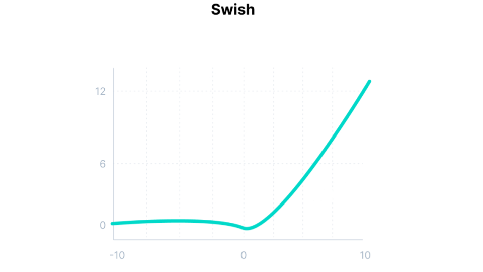
Fig. 53 . The Swish activation function.
_{Image: www.v7labs.com}

The Swish function exhibits increased classification accuracy and consistently matches or outperforms ReLU activation function on deep networks (especially on image classification).

Pros

• It is differentiable on the whole range

• The function is smooth and non-monotonic (like GELU), which is an advantage to enhance input data during learning

• Unlike the ReLU function, small negative values are not zeroed, allowing for a better modeling of the data. And large negative values are zeroed out (in other words, the node will die only if it needs to die)

Cons

• More a warning than a con: the Swish function is only relevant if it is used in neural networks having a depth greater than 40 layers

How to choose the right activation function

The risk of vanishing or exploding gradients

Training a neural network with a gradient-based learning method (the gradient descent is one) can lead to issues. The culprit, or rather cause, lies in the choice of the activation function:

Vanishing Gradient problem
As seen with the sigmoid and hyperbolic tangent, certain activation functions converge asymptotically towards the bounded range. Thus, at the extremities (large negative or large positive input values), a large change in the input will cause a very small modification of the output: there is a saturation. As a consequence the gradient will be also very small and the learning gain after one iteration very minimal, tending towards zero. This is to be avoid if we want the algorithm to learn a decent amount at each step.

Exploding Gradient problem If significant errors accumulate and the neural network updates the weights with larger and larger values, the difference between the prediction and observed values will increase further and further, leading to exploding gradients. It’s no more a descent but a failure to converge. Pragmatically, it is possible to see it when weights are so large that they overflow and return a NaN value (meaning Not A Number).

(Generic) tips

The first tip would be: it all depends on the task at hand. Of course this may leave you confused now. Here is the corrollary of the first tip: practice, practice, practice (and some reading). You will soon explore existing neural networks, build your own and experiment different functions to see which one is more appropriate. Yes, there is a bit of tweaking involved with your organic brain to train an artificial one! More on this in the Lecture “Towards Deep Learning Modeels.”

The second one tip would be: in doubt, opt for ReLU for the hidden layers. It is the most successful and widely-used activation function. Although the rectifier variants have tried to improve it, the ReLU remains the top contender among activation function for the hidden layers. And it is a very fast computation, another point to start optimizing your neural network with it.

Usually, all hidden layers usually use the same activation function. For the final layer however, the sigmoid or tanh are usually preferred, in particular in classification. For multiclass, an adapted version of the sigmoid is the Softmax function. It is a combination of multiple sigmoids with outputs summing to one, outputing the relative probabilities or each class.

The platform paperswithcode.com aims at sharing Machine Learning papers along with code, dataset and evaluation tables; all open source and free. There are also dedicated portals for Mathematics, Statistics, Computer Science, Physics and Astronomy.

Learn More

• Neural Network Activation Functions Cheat-sheet from v7labs.com

• Summary table on Wikipedia: article on Activation Functions

• List of Activation Functions on the website Paper With Code