Linear Regression in Python
Contents
1. Linear Regression in Python#
Learning Objectives
In this tutorial, you will learn how to code a linear regressor in python. The steps will be detailed and the present document will show you basic commands in python to get started.
Main goals:
Code a linear regressor to fit a dataset of one independent variable with its target
Display visualization of the gradient descent
What will also be covered:
How to load and explore a dataset
How to plot with Matplotlib
How to define custom functions
How to printout and store intermediary results
How to structure and comment code
Warning
Boring alert!
You have coded before and you are done already?
Come talk to me, I will give you extra challenges.
Let’s now open a fresh Jupyter Notebook on Colaboratory and follow along! To create a blank Colaboratory document, go to your GDrive first. On the top left of the screen there is a “+” button. Click on it, the drop menu will show several options with “More” at the bottom: hover it and you will see another drop down menu where you can click on Colaboratory.
1.1. Get the data#
The first step is to get the dataset. It can be accessed here. We will see how to localize, explore and load it.
1.1.1. Connect#
First, get to the shared folder, right click on the .csv file and select “Add shortcut to Drive.” This will allow you to access the folder from your drive!
Then in your Colaboratory tab, write and execute the following lines:
from google.colab import drive
drive.mount('/content/gdrive')
1.1.2. Localizing the file#
In Jupyter Notebook, it is possible to write bash commands (the language used in a console, or terminal) by appending a ! at front of a code cell.
The pwd command stands for “print working directory” and will show you were you are currently running your code.
!pwd
To list files, use the ls command of ls -l to display more details:
!ls -l
Tip
Once you locate where your data file is in your drive, it is a good practice to store its path, i.e. the string of character matching all the directory and subdirectories, in a variable (usually named path).
1.1.3. Exploring the file#
Often you will not know how data is presented in a file. In bash, the cat command will display the entire content of a text file. But caution: your file can have thousands of lines! What is usually relevant to see is e.g. if the file has a header row. The command that displays the first rows is head. By default it will show 10 rows, but you can tweak this number with the -n option:
!head -n 5 ../data/tutorial_1.csv
x,y
5.4881350392732475,29.65450786127179
7.151893663724195,34.99358978951999
6.027633760716439,35.99427342345802
5.448831829968968,24.815775427356154
Too see how many lines your file has, use the “word count” command wc with the -l option for line:
! wc -l ../data/tutorial_1.csv
51 ../data/tutorial_1.csv
This is useful to know which amount of data we are dealing with.
And we also see the file has a header row. Let’s now load its content in a pythonic way.
1.1.4. From csv to dataframe#
A dataframe is a data structure from the pandas software library designed for tabular data. It can be compared to an array with rows and columns that can be modified in an intuitive way for the programmer. Pandas allows importing data from various file formats. There is a special method for loading the content from a .csv file:
import pandas as pd

filename = "../data/tutorial_1.csv"
df = pd.read_csv(filename)
df.head()
| x | y | |
|---|---|---|
| 0 | 5.488135 | 29.654508 |
| 1 | 7.151894 | 34.993590 |
| 2 | 6.027634 | 35.994273 |
| 3 | 5.448832 | 24.815775 |
| 4 | 4.236548 | 21.034960 |
Jupyter Notebook offers a nice display of tabular data structure, with indexed rows and column names. It’s very convenient to explore a file. However even the head method can not fit in the terminal if the file contains lots of columns (features). It’s possible to print the columns names using the keys command: df.keys().
1.1.5. From dataframe to NumPy arrays#
Let’s now store each column into a python list, as it will be handy for plotting and coding our regressor. Python has lists but we will use a more advanced object from the NumPy library, which is efficiently coded to perform mathematical operations on multi-dimensional arrays and matrices. This will store each column as a NumPy array:
import numpy as np

x = df['x'].to_numpy()
y = df['y'].to_numpy()
len(x)  # print number of elements
50
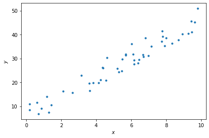
1.2. Plot the data#
Let’s use the matplotlib.pyplot library to make a scatter plot of the data:
import matplotlib.pyplot as plt

fig, ax = plt.subplots()
ax.scatter(x, y, s=10)
ax.set_xlabel('$x$')
ax.set_ylabel('$y$')
plt.tight_layout()
1.3. Writing functions#
We will have to make the same computations several times, for instance while calculating the hypothesis function. Thus it is better to define proper functions for that. Here is a demo with the hypothesis function:
def h_lin(theta_0, theta_1, x):
    return theta_0 + theta_1 * x
Your first mission is to write a function calculating the cost \(J(\theta_0, \theta_1)\).
Good Practice
Before even starting to write code it is important to be very clear on what are the inputs, the main steps, the outputs. I recommend going back to the ‘pen and paper’ to first write the algorithm, list the different variables. Then it will make the coding much easier and less error-prone.
There will be another handy function to code. Recall the derivative of the cost function. It contains the difference between the predicted value and the observed one, without them being squared. This difference has the technical name of “residual”. You will write another function get_residuals() computing the residuals, which is common in both partial derivatives \(\frac{\partial J(\theta_0, \theta_1)}{\partial \theta_i}\).
Questions are summarized at the end of the document for convenience. Hints will be given during the tutorial to guide you.
Test your code
Once you have your function computing the cost, it is always a good practice to test it. Let’s take the values seen in class from the plot of the Perfectly aligned 4 points. Use your function to check that the cost is zero for \(\theta_1\) = 2. You will have to complete it with the proper variables to pass to the cost function (instead of the ... placeholder):
x_test = np.array([1, 2, 3, 4])
y_test = np.array([2, 4, 6, 8])

# No intercept term
theta_0 = 0

# List of values for theta 1:
theta_1_vals = [0, 0.5, 1, 1.5, 2, 2.5, 3, 3.5]

for ... in ... :
    cost = costFunctionLinRegression( ... )
    print(f"With theta 1 = {theta_1:.1f}\tcost = {cost:.2f}")
Let’s now get to the core of things: the regressor!
1.4. Linear regressor#
A skeleton of the code is given below to help you get started. You will have to tweak the hyperparameters and initial \(\theta\) parameters.
# Hyperparameters
alpha =
N =

# Initialization
theta_0 =
theta_1 =

# Check lists of x and y are of same length:
m = len(x) # sample size
if m != len(y): raise ValueError('The lists of x and y values are not the same length!')

# Store theta (weights) values for Gradient Descent (GD) visualizations
GD_all_thetas_0 = np.array([theta_0])
GD_all_thetas_1 = np.array([theta_1])

print("Starting gradient descent\n")

# -------------------
#   Start iterations
# -------------------
for n in range(1, N+1):

    #___________________________

    # Your code here


    #___________________________

print(f"\nEnd of gradient descent after {n} iterations")
1.5. Printouts#
While in the process of writing code and testing its parts, it is good to print in the terminal some values for checks. But not all the values for each iteration! There will be too many lines in the terminal and it will be difficult to see the trend (if the gradient converges or not).
To print selected values, e.g. every 100 iterations, use the modulo % operator:
for i in range (1,501):
    if i%100 == 0:
        print(f"Iteration {i}")
Iteration 100
Iteration 200
Iteration 300
Iteration 400
Iteration 500
You may have to display values more often at the beginning, as the gradient descent will work its way quite fast towards a good approximation of the optimized parameter values, then the rest of the iterations will be refining those values.
1.6. Visualization of Gradient Descent#
Let’s reproduce the plots from the lecture, Figure Fig. 13 to visualize the trajectory of the gradient descent in the theta parameter space.
1.6.1. Storing intermediary parameter values#
For this you will have to append to the lists weights_GD_0 and weights_GD_1 the intermediary theta values.
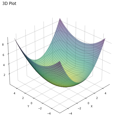
1.6.2. Plotting macros 3D and contour#
Below are examples on how to make a 3D plot and a contour plot for inspiration.
# Generating data input points
xlist = np.linspace(-5.0, 5.0, 100)
ylist = np.linspace(-5.0, 5.0, 100)
X, Y = np.meshgrid(xlist, ylist)

# Creating elliptical plane
Z = (X**2)/4 + (Y**2)/9

fig = plt.figure(figsize=(8, 8))
ax = fig.add_subplot(111, projection='3d')

# Drawing contour plot
surf = ax.plot_surface(X,Y,Z, cmap='viridis_r', linewidth=0.3, alpha = 0.5, edgecolor = 'k')

# Set plot and axis titles (and white background)
plt.title('3D Plot', loc='left', fontsize = 15)
ax.set_xlabel('X'); ax.xaxis.set_pane_color((1.0, 1.0, 1.0, 0.0))
ax.set_ylabel('Y'); ax.yaxis.set_pane_color((1.0, 1.0, 1.0, 0.0))
ax.set_zlabel('Z'); ax.zaxis.set_pane_color((1.0, 1.0, 1.0, 0.0))

# To change plot view angle
ax.azim = 225
ax.elev = 30
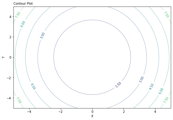
The 2D representation of this 3D plot above can be coded this way:
fig, ax = plt.subplots(figsize= (9, 6))

CS = ax.contour(X,Y,Z, linewidths=0.5)
ax.clabel(CS, CS.levels[0:10], inline=1, fontsize=10, fmt='%.2f')
ax.set_xlabel('X')
ax.set_ylabel('Y')
plt.title('Contour Plot', loc='left', fontsize = 10)

fig_width, fig_height = plt.gcf().get_size_inches()
1.7. Summary of the mission#
Here is a summary of your mission:
Functions
Write a function calculating the cost \(J(\theta_0, \theta_1)\)
Write a function calculating the residuals \(y^\text{pred} - y^\text{obs}\)
Test your functions to check they run and compute the right thing
Take the linear regressor skeleton and complete the
forloopList the main steps (pen and paper!)
Call the functions
Implement printouts of relevant variables
Visualize the gradient descent
Modify your regressor to store intermediary \(\theta\) parameter values
Plot the 3D visualization of the cost vs \(\theta_0\) and \(\theta_1\)
Add the stored intermediary \(\theta\) parameter values (use the
plotmethod)Plot the 2D contour of the cost vs \(\theta_0\) and \(\theta_1\)
Add the stored intermediary \(\theta\) parameter values (use the
plotmethod)
Bonus: compare with SciPy optimizer
The SciPy library contains numerous mathematical tools, including an optimizer. You can use the code to get the optimized \(\theta\) values and compare with the ones you found with your linear regressor:
def residuals_func(v, x, y):
    return y - (v[1]*x+v[0])

res = scipy.optimize.least_squares(residuals_func, x0=[0, 0], args=(x,y))
print(f"SciPy MSE optimizer best-fit line: {res.x[1]:.3f} X + {res.x[0]:.3f}")