What is boosting?

Definitions

The general idea behind boosting is a correction of previous learners by the next row of classifiers.

Definition 48

Boosting refers to ensemble methods that are tuning weak learners into a strong one, usually sequentially, with the next predictor correcting its predecessors.

Usually the predictors are really shallow trees, namely one root nodes and two final leaves. This has a name:

Definition 49

A decision stump is a one-level decision tree. It has one root node evaluating only one input feature and the two resulting branches immediately connect to two terminal nodes, i.e. leaves.

Many boosting methods are available. We will see two popular ones: AdaBoost and Gradient Boosting.

AdaBoost

Algorithm

AdaBoost is short for Adaptative Boosting. It works by assigning larger weights to data samples misclassified by the previous learner. Let’s see how this work.

Algorithm 4 (AdaBoost)

Inputs
Training data set \(X\) of \(m\) samples

Outputs
A collection on decision boundaries segmenting the \(k\) feature phase space.

Initialization
Each training instance \(x^{(i)}\) is given the same weight

\[\begin{equation*} w^{(i)} = \frac{1}{m} \end{equation*}\]

Start
For each predictor \(j = 1 , \cdots , N^\text{pred}\)
a. Train on all samples and compute the weighted error rate \(r_j\)

(35)\[\begin{equation} r_j = \frac{\sum_{i = 1}^m w^{(i)} [ \hat{y}_j^{(i)} \neq y^{(i)} ] }{\sum_{i = 1}^m w^{(i)}} \end{equation}\]

b. Give the predictor \(j\) a weight \(W_j\) measuring accuracy

(36)\[\begin{equation} W_j = \alpha \log \frac{1 - r_j}{r_j} \end{equation}\]

\(W_j\) points to a high number if the predictor is good, zero if the predictor is guessing randomly, negative if it is bad. \(\alpha\) is the learning rate.

c. Update the weights of all data samples:

(37)\[\begin{equation} w^{(i)} = \left\{\begin{matrix} w^{(i)} \;\;\;\; &\text{if} \;\;\;\; \hat{y}_j^{(i)} = y_j^{(i)} \\[2ex] \;\;w^{(i)} \exp (-W_j) \;\;\;\; &\text{if} \;\;\;\; \hat{y}_j^{(i)} \neq y_j^{(i)} \\ \end{matrix}\right. \end{equation}\]

d. Normalize the weights

(38)\[\begin{equation} w^{(i)} \rightarrow \frac{w^{(i)}}{\sum_{i = 1}^m w^{(i)}} \end{equation}\]

Exit conditions

• \(N^\text{pred}\) is reached

• All data sample are correctly classified (perfect classifier)

The illustration below gives a visual of the algorithm.

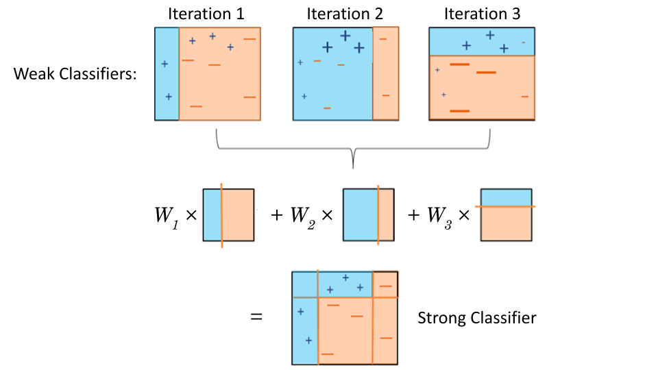
Fig. 35 . Visual of AdaBoost.
Misclassified samples are given a higher weight for the next predictor.
Base classifiers are decision stumps (one-level tree).
_{Source: modified work by the author, originally from subscription.packtpub.com}

Note

As the next predictor needs input from the previous one, the boosting is not an algorithm that can be parallelized on several cores but demands to be run in series.

How does the algorithm make predictions? In other words, how are all the decision boundaries (cuts) combined into the final boosted learner?

The combined prediction is the class obtaining a weighted majority-vote, where votes are weighted with the predictor weights \(W_j\).

(39)\[\hat{y}(x^\text{new}) = \arg\max_k \; \; \sum_{j = 1}^{N^\text{pred}} W_j \;[\; \hat{y}_j(x^\text{new}) = k \;]\]

The argmax operator finds the argument that gives the maximum value from a target function. The expression in square braket is a condition on the sum. There are as many sums as classes \(k\), going over all predictors \(j\). The predicted class is the one having the largest sum.

Implementation

In Scikit-Learn, the AdaBoost classifier can be implemented this way (sample loading not shown):

from sklearn.ensemble import AdaBoostClassifier

ada_clf = AdaBoostClassifier( 
    DecisionTreeClassifier(max_depth=1),
    n_estimators=200,
    algorithm="SAMME.R",
    learning_rate=0.5)

ada_clf.fit(X_train, y_train)

The decision trees are very ‘shallow’ learners: only a root note and two final leaf nodes (that’s what a max depth of 1 translates to). But there are usually a couple of hundreds of them. The SAMME acronym stands for Stagewise Additive Modeling using a Multiclass Exponential Loss Function. It’s nothing else than an extension of the algorithm where there are more than two classes. The .R stands for Real and it allows for probabilities to be estimated (predictors need the option predict_proba activated, otherwise it will not work). The predictor weights \(W_j\) can be printed using ada_clf.estimator_weights_.

Learn More

• AdaBoost on Scikit-Learn

• AdaBoost, Clearly Explained - StatQuest video on YouTube

• A comparison between a decision stump, decision tree and AdaBoost SAMME and SAMME.R from Scikit-Learn.org

Gradient Boosting

The gradient is back!

Core concept

Contrary to AdaBoost, which builds another decision stump based on the errors made by the previous decision stump, Gradient Boosting starts by making a single leaf. This leaf represents an initial guess (round 0). Next, a first tree is made, outputting a first round of predictions (round 1). Then the pseudo-residuals are calculated. They are residuals, in the sense that they are the difference, for each training sample, between the predicted class and the observed class. We will see how this is computed from a binary output to a probability soon. The key concept behind Gradient Boosting is that the next tree fits the residuals of the previous one. In this sense, Gradient Boosting is performing a gradient descent, the residuals giving the step direction to go to minimize the errors and thus improve the prediction’s accuracy. Final predictions are made by ‘summing the trees’ (times a learning rate) and converting the final number into a probability for a given class.

We will go through an example with a very small dataset to understand the steps and calculations.

A minimal example

Let’s say we have a dataset of simulated training samples of collisions and for each collision some features such as an invariant mass and missing transverse energy (these variables will be explained during tutorials). We want to use Gradient Boosting to search for new physics. This new physics process is simulated in signal samples (target \(y=1\)) and background processes, i.e. interactions from known physics processes but mimicking the signal outputs, are with \(y=0\).

Row	\(m_{bb}\)	MET	…	Class
0	60	35	…	0
1	110	130	…	1
2	45	78	…	0
3	87	93	…	0
4	135	95	…	1
5	67	46	…	0

Step 0: Initial Guess
We start by an initial guess. In Gradient Boosting for classification, the initial prediction for every samples is the log of the odds. It is an equivalent of the average for logistic regression:

(40)\[\text{log(odds) } = \log \frac{N[y=1]}{N[y=0]} \]

Here we have 2 signal events and 4 background ones, so log(odds) = \(\log \frac{2}{4}\) = -0.69

How to proceed now with classification? If you recall logistic regression, the binary outcomes were converted as an equivalent of a probability with the logistic function (sigmoid). We will use it again here:

(41)\[\text{ Probability of signal } = \frac{1}{1 + e^{- \text{log(odds)}}} \]

In our example, \(\frac{1}{1 + e^{ - \log \frac{2}{4} }} = \frac{1}{3}\).

Step 1: pseudo residuals
Now let’s calculate the pseudo residuals.

Definition 50

Pseudo residuals are intermediate errors terms measuring the difference between the observed values and an intermediate predicted value.

\[\begin{equation*} \text{Pseudo residuals} = ( \text{Observed} - \text{Prediction} ) \end{equation*}\]

We will store pseudo residuals as an extra column. For the first row (index 0), the pseudo residual is \(( 0 - \frac{1}{3}) = -\frac{1}{3}\). The second, with observed value 1, is \(( 1 - \frac{1}{3}) = \frac{2}{3}\).

Row	\(m_{bb}\)	MET	…	Class	Residuals
0	60	35	…	0	-0.33
1	110	130	…	1	0.67
2	45	78	…	0	-0.33
3	87	93	…	0	-0.33
4	135	95	…	1	0.67
5	67	46	…	0	-0.33

Step 2: tree targeting the pseudo residuals
Now let’s build a tree using the input features but to predict the residuals.

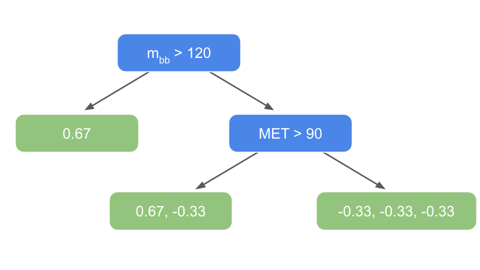
Fig. 36 . First tree predicting the residuals.
_{Image from the author}

The tree is very minimal because we only have six samples in the dataset! Usually there can be up to 32 leaves in Gradient Boosting intermediary trees.

Step 3: leaves’ output values
The predictions are in terms of the log of the odds, whereas leaves are derived from a probability. We will have to translate the residuals in the leaves above as “log of the odds” first. Only after getting the correct leave outputs can we combine trees together. When using Gradient Boost for classification, the most common transformation is the ratio:

(42)\[\frac{ \sum \text{Residuals}_i }{\sum [ \text{Previous Probability}_i \times ( 1 - \text{Previous Probability}_i )]}\]

The numerator is the sum of residuals in a given leaf \(i\). The denominator is the product of the previously predicted probabilities for each residual in that same leaf \(i\). Let’s illustrate with our example. For the leaf on the very left, there is only one residual (from sample row 4) of 0.67 with an associated probability of \(\frac{1}{1 + \exp( - \log \frac{2}{4} )} = \frac{1}{3}\). So:

(43)\[\frac{\frac{2}{3}}{ \frac{1}{3} \times ( 1 - \frac{1}{3})} = 3\]

The new output value for the leaf is 3. Now the second leaf from the left has two samples in it: rows 1 and 3. The former is signal, with a residual of \(\frac{2}{3}\) and an associated (previous) probability of \(\frac{1}{3}\), whereas the latter is a background sample with a residual of \(-\frac{1}{3}\) and associated probability of \(\frac{2}{3}\).

(44)\[\frac{ \frac{2}{3} -\frac{1}{3}}{ \frac{1}{3} \times ( 1 - \frac{1}{3}) + \frac{2}{3} \times ( 1 - \frac{2}{3})} = \frac{3}{4} = 0.75\]

For the last leaf, we have:

(45)\[\frac{-\frac{1}{3} -\frac{1}{3} -\frac{1}{3}}{ \frac{2}{3} \times ( 1 - \frac{2}{3}) + \frac{2}{3} \times ( 1 - \frac{2}{3}) + \frac{2}{3} \times ( 1 - \frac{2}{3})} = -\frac{3}{2} = -1.5\]

The tree has now output values:

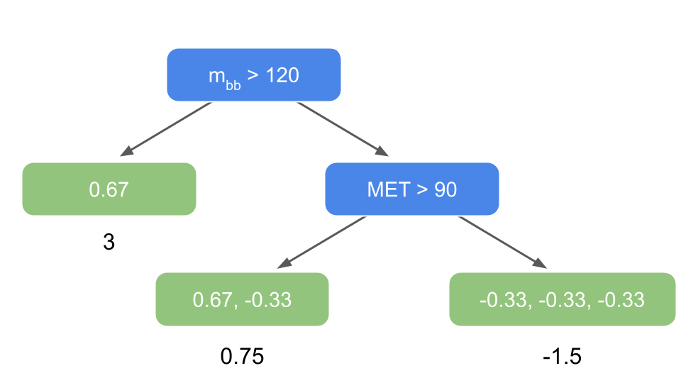
Fig. 37 . First tree predicting the residuals with output values for each leaves as ‘predictions’ (log of odds).
_{Image from the author}

Step 4: update predictions
The first tree targeting the residuals is combined with the initial guess:

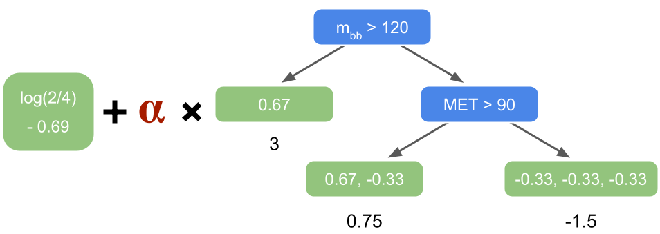
Fig. 38 . The initial guess and the first tree are combined. The tree is scaled by a learning rate \(\alpha\).
_{Image from the author}

Usually the learning rate is around 0.1 but for simplicity here in our example, we will take a larger value of \(\alpha = 0.5\) (to get a more drastic change after only two rounds). The first row of index 0 falls into the right leaf. To calculate the new log of the odds prediction for row 0, we sum the initial guess with the learning rate times the leaf output (expressed as a log of the odds from the calculation above):

(46)\[\text{log(odds) Prediction row 0} = - 0.69 + {\color{Mahogany}\alpha} \times (-1.5) = - 0.69 + {\color{Mahogany}0.5} \times (-1.5) = -1.44\]

Now we convert the new log of the odds as a probability:

(47)\[\text{ Probability row 0 } = \frac{1}{1 + e^{- (-1.44) }} = 0.19\]

As this row 0 is a background event, we went from an initial guess of probability \(\frac{1}{3}\) to now 0.20, which is closer to zero, so our first residual-fitted-tree added a correction in the right direction. Let’s take row 1 now. It lands in the middle leaf. Thus:

(48)\[\text{log(odds) Prediction row 1} = - 0.69 + {\color{Mahogany}\alpha} \times 0.75 = - 0.69 + {\color{Mahogany}0.5} \times 0.75 = -0.315\]

The probability is:

(49)\[\text{ Probability row 0 } = \frac{1}{1 + e^{- (-0.315) }} = 0.42\]

The event is signal, so our prediction should be close to 1. We went from an initial guess probability of \(\frac{1}{3}\) to 0.42. We indeed go in the right direction! Smoothly, but surely.

Note

It has been shown empirically that a slow learning rate is preferrable to reach a good accuracy. It comes at the price of having to build numerous intermediary trees incrementing the predictions in small steps. Without a learning rate scaling the trees, there is a high risk to stay too close to the data, which would bring a low bias but very high variance. Thanks to a small learning rate, taking lots of small steps in the right direction results in better predictions with a testing dataset. This technique is called shrinkage.

We can add an extra column with the predicted probabilities (pred prob) in our dataset table:

Row	\(m_{bb}\)	MET	…	Class	Residuals	Pred Prob
0	60	35	…	0	-0.33	0.19
1	110	130	…	1	0.67	0.42
2	45	78	…	0	-0.33	0.19
3	87	93	…	0	-0.33	0.42
4	135	95	…	1	0.67	0.69
5	67	46	…	0	-0.33	0.19

We can see that the predicted probabilities for background went towards zero, whereas those for signal got incremented towards 1.

Step 2bis: new pseudo residuals We go back to step 2 to compute the new pseudo residuals from the last set of predictions. Then the step 3 will consist of building a second tree targeting those new residuals. Finally, one we have all the output values for the resulting tree leaves, we can add the second tree to the initial guess and the first tree (also scaled with the learning rate).

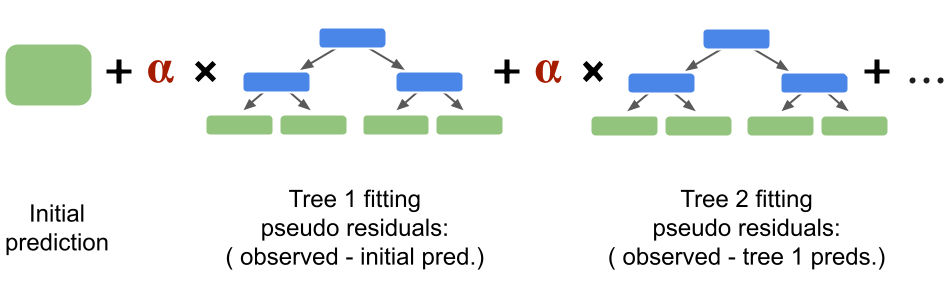
Fig. 39 . The Gradient Boosting sums the trees fitting the pseudo residuals from the previous predition.
_{Image from the author}

The process repeats until the number of predictors is reached or the residuals get super small.

Predictions on test samples

How are predictions made on new data? By simply using the sum above. We run the new sample in the first tree, get the output value of the leaf in which the sample ends up, then run it through the second tree, get the final leaf output value as well. The final prediction is done computing the sum with the initial prediction and each tree prediction scaled by the learning rate. If it is greater than 0.5, the class is signal: \(y^\text{pred} = 1\). If lower, we predict the sample to be background.

Implementation

Scikit-Learn has two classes implementing Boosting: GradientBoostingRegressor (for regression, see below some links covering it if you are curious) and GradientBoostingClassifier. The latter supports multi-class classification. The main hyperparameters are the number of estimators n_estimators (how many intermediary trees are built) and the learning_rate \(\alpha\).

from sklearn.model_selection import train_test_split
from sklearn.ensemble import GradientBoostingClassifier

# Getting the dataset [sample loading not shown]
X_train, X_test, y_train, y_test = train_test_split(X, y, test_size=0.2, random_state=42)

# Creating the Gradient Boosting (GB) classifier:
gb_clf = GradientBoostingClassifier(
    n_estimators=100, 
    learning_rate=1.0, # no shrinkage here, otherwise 0.1 is a common value
    max_depth=1, # here decision stumps
    random_state=0)

gb_clf.fit(X_train, y_train)

# Printing score (accuracy by default)
gb_clf.score(X_test, y_test)

The size of each intermediate tree can be controlled by max_depth (it is rarely a stump, rather a tree of depth 2 to 5) or max_leaf_nodes. There are different log functions available, the log-loss being the default.

Note

The classes above have been superseeded by HistGradientBoostingRegressor and HistGradientBoostingClassifier. They are inspired by the framework LightGBM for Light Gradient Boosting Machine, developed by Microsoft. Histogram-based estimator will run orders of magnitude faster on dataset larger than 10,000 samples. More information on Scikit-Learn Historgram-Based Gradient Boosting.

XGBoost the warrior

XGBoost, for eXtreme Gradient Boosting, is a software library offering a fully optimized implementation of gradient boosting machines, focused on computational speed and model performance. It was created in 2016 by Tianqi Chen, at the time Ph.D. student at the University of Washington. XGBoost gained significant popularity in the last few years as a result of helping individuals and teams win virtually every Kaggle structured data competition, and in particular the Higgs Boson Machine Learning Challenge.

In terms of model features, XGBoost has the standard Gradient Boosting, as well as a Stochastic Gradient Boosting (more on this Lecture 7) and a Regularized one (with both L1 and L2 regularization methods).

It has also system features. Parallelization (to efficiently construct trees using all available CPU cores), Distributed Computing (if working with a cluster of machines), Out-of-Core Computing (when very large datasets can’t be loaded entirely in the memory), Cache Optimization (to minimize the need to access data in underlying slower storage layers).

The algorithm features contains some technical jargon. Here is a selection of the main ones with some explanations:
Sparsity Awareness Data is considered sparse when certain expected values in a dataset are missing, or with mostly the same value, which is a common phenomenon in general large scaled data analysis. This can alter the performance of machine learning algorithms. XGBoost handles sparsities in data with the Sparsity-aware Split Finding algorithm that choose an optimal direction in the split, where only non-missing observations are visited.
Block Structure Data is sorted and stored in in-memory units called blocks, enabling the data layout to be reused by subsequent iterations instead of computing it again.
Continued Training XGBoost makes it possible to further boost an already fitted model on new data, without having to reload everything.

Here is a minimal example of implementation in Python as well as other languages.

arXiv is a free distribution service and an open-access platform for more than two million scholarly articles in the fields of physics, mathematics and computer science among others. Some articles are submitted to journals (peered-review) but others are not peered-reviewed. It is possible to subscribe and receive a selection of newly submitted articles in your mailbox: To Subscribe to the E-Mail Alerting Service

Exercise

It is always good to ‘go to the source,’ i.e. the original papers. Yet this can be over-technical and daunting.

Here is the paper of XGBoost on the arXiv platform: XGBoost: A Scalable Tree Boosting System, paper on arXiv (2016)

To make it more enriching and fun, dive into the paper with a classmate. After each section, take turns to explain to your peer what you understand with your own words. This will train you to read the literature in the future, be confronted to different mathematical notations and digest the content (papers are usually dense in information, so don’t worry if it takes you time to go through it).

In the tutorial, we will classify collision data from the Large Hadron Collider using decision trees, then a random forest and finally boosted classifiers. We will compare their performance with the metrics introduced in Lecture 3.

Learn More

Gradient Boosting
Gradient Tree Boosting in Scikit-Learn
AdaBoost Tutorial on Kaggle

StatQuest series on Gradient Boost (with Josh Starmer and his humour)
Gradient Boost Part 1: Regression Main Ideas video
Gradient Boost Part 2: Regression Details video
Gradient Boost Part 3: Classification video
Gradient Boost Part 4: Classification Details video

XGBoost
Documentation Read The Docs
XGBoost: A Scalable Tree Boosting System, paper on ArXiv (2016)
Tianqi Chen provides a brief and interesting back story on the creation of XGBoost in the post Story and Lessons Behind the Evolution of XGBoost.