T5. Neural Network by Hand!
Contents
T5. Neural Network by Hand!#
In this tutorial, you will code a little neural network from scratch. Don’t worry, it will be extremely guided. The two most important points being that you learn and you have fun.
For programmers already fluent in Python
If you have had some programming experience already, please stick to the code template below for evaluation purposes. Afterwards, feel free to append to your notebook a more elaborate code (see Parts II and III).
We’ll use the network to solve the classic XOR problem. This is how the data look like:
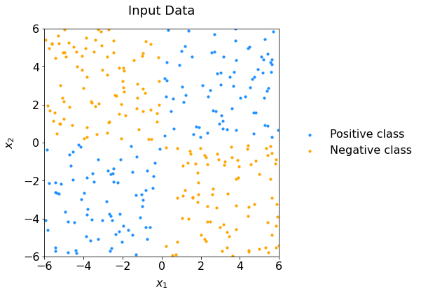
Fig. 62 Scatter plot of data representing the XOR configuration: it is not linearly separable.#
Part 0: The Math#
As a warm-up, you are asked to derive Equations (117), (125) – (130) from the section on the Backpropagation Algorithm. In class, you saw the main blocks. Here, it is about working out the indices to see which exact tensor operations are being used.
Remember that a matrix element \(w_{jk}\) of a matrix \(W\) becomes \(w_{kj}\) once it is transposed as \(W^\top\).
The outer product of two vectors \(a \otimes b\) can also be written as: \(a \; b^\top\) .
Refrain from using indices already taken in the course (\(i\), \(\ell\), \(m\), \(n\)) to avoid confusion with sample index, layer number, total number of samples and number of features, respectively. Lots of other letters are available 😉.
Part I: Code Your Neural Network!#
1.0 Setup#
Copy the code from the Setup in Appendix: T5 Snippet Zone into a fresh Colaboratory notebook.
Advice
Read everything first before starting
1.1 Get the Data#
1.1.1 File Download#
Retrieve the files:
ml_tutorial_5_data_train.csv
ml_tutorial_5_data_test.csv
1.1.2 Split Signal vs Background#
Create a sig and bkg dataframes that collect the real signal and value samples. We will need this later on.
Hint: we did this already in Tutorial 3.
1.1.3 Dataframe to NumPy#
Declare the following variables to store the dataset into NumPy arrays:
inputs = ['x1', 'x2']
X_train =
y_train =

X_test =
y_test =
1.2 Functions#
1.2.1 Weighted Sum#
Create the function z that compute the weighted sum of a given activation unit, as seen in class. You do not have to worry about the dimensions of objects here, this will come later. Make sure the names of the arguments are self-explanatory:
def z( ... , ... , ... ):
    #...
    return #...
1.2.2 Activation Functions and Derivatives#
Write the hyperbolic tangent and sigmoid activation functions, followed by their derivatives:
def tanh(z):
    return #...

def sigmoid(z):
    return #...

def sigmoid_prime(z):
    return #...

def tanh_prime(z):
    return #...
1.2.3: Cross-entropy cost function#
Write the cross-entropy cost function.
def cross_entropy_cost(y_pred, y_true):
    #...
    return #...
1.2.4 Derivative of the Loss#
As seen in class, the loss function for classification is defined as:
Find the expression of:
Use a text cell and LaTeX. If you are new to LaTeX, this application will help. Once you have an expression for the derivative of the loss, code it in python:
def L_prime(y_pred, y_true):
    #...
    return #...
1.3 Feedforward Propagation#
It is time to write the feedforward function!
We will start with the following network for now:
The network has two hidden layers
The nodes of the hidden layers use the hyperbolic tangent as activation function
The output layer uses the sigmoid function
1.3.1 Implementing the Feedforward Function#
The number of activation units in each layer is dynamic. Your code should work with tensors \((i, j, k)\) with \(i\) the index referring to the \(i\)th sample, \(j\) the index of the activation unit and \(k\) here should be 1, as we consider a column vector. The weights and biases are given as input, stored in lists. The input data has been reshaped for your convenience (and a bit less of debugging time 😉).
Complete the function below that does the feedforward propagation of the network, using the equations shown in class. Look at the output to see how to name your variables!
def feedforward(input_X, weights, biases):
    W1, W2, W3 = weights
    b1, b2, b3 = biases

    m  = len(input_X)
    a0 = input_X.reshape((m, -1, 1))

    # First layer
    z1 = ...
    a1 = ...

    # Second layer
    z2 = ...
    a2 = ...

    # Third layer
    z3 = ...
    a3 = ...

    nodes = [a0, z1, a1, z2, a2, z3, a3]
    return nodes
Check Point 1
At this point in the assignment, it is possible to ask for a checkup with the instructor before moving forward to …the backward pass (pun intended).
Send an email to the instructor with the exact title [Intro to ML 2025] Tutorial 5 Check 1, where you paste your completed code of your weighted sum (question 1.2.1) and the feedforward function above (question 1.3.1).
⚠️ Do not send any notebook!
1.3.2 Predict#
The predict function is already provided in the setup. Your task is to think about how it works:
What is the
output_nodein our 2-hidden-layer neural network?What kind of values does
predictreturn?After running
feedforward, how would you callpredictto get predictions?
Keep your answers short and clear.
1.4 Neural Network Training#
Time to train! Copy paste the code in Train: Skeleton as your starting point. To help you further, hyperparameters are given. Replace the #... with your own code.
Weight Initialization
The weight matrices and bias vectors can be simply initialized with a random number between 0 and 1. Use:
an_i_by_j_matrix = np.random.random(( i , j ))
The double parenthesis is important to get the correct shape. To make your code modular, use the variables encoding the number of activation nodes on the first and second hidden layers.
Feedforward and Predict
To return the last element of a list:
my_list[-1]
Matrix / Vector Operations
In Python, matrix multiplication is done using @.
Element-wise multiplication is done using *.
Transposing Tensors
To transpose a matrix
M:M.T
To transpose 3D arrays, reorder indices:
np.transpose(my3Darray, (0, 2, 1))
Summing Tensors
To sum all elements:
np.sum(my_array)
To sum a 3D array on the first index:
np.sum(my3Darray, axis=0)
In general, use the
axisargument to choose which dimension(s) to reduce.
Check Point 2
If your code runs without errors, you may inform the instructor of your progress by sending an email titled [Intro to ML 2025] Tutorial 5 Check 2.
Paste your training loop in the email, and attach a text file containing the cell output.
⚠️ Do not send any notebook!
1.5 Plots#
1.5.1 Cost evolution#
Call the provided function plot_cost_vs_iter in the Setup to plot the cost evolution of both the training and testing datasets.
1.5.2 Scatter Plot#
Use the get_decision_surface and plot_scatter functions (in Setup) to visualize the decision boundaries of your trained neural network. Did your neural network successfully learn the XOR function?
If all goes well, you should obtain something like this:
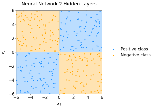
Fig. 63 Scatter plot of data representing the XOR configuration and the neural network performance.#
You just coded a neural network by hand!
Part II: Vectorize Your Neural Network#
We coded everything for two hidden layers only. Let’s make it more general. But in two steps:
2.1 Dynamic Depth#
Modify your code so that it creates a network of dynamic depth. You can encode the architecture as an array. For instance:
layers = [3, 3, 2, 1]
would create a network of four layers with three activation units on the first and second layers, two on the before-last hidden layer and the output layer would have one node. To make things easier, keep one output node in the last layer for now.
Good luck!
2.2 Several Output Nodes#
Modify your code further to have more than one output node in the last layer. You may have to change your cost function with the categorical cross-entropy. Feel free to create toy datasets with more than two classes. Or pick-up some of Scikit-Learn datasets!
Part III: Play!#
3.1 Momentum et all#
Implement by hand some momentum. The action is in your update rule after you backpropagate. Try to come up with plots to visualize the convergence. Discuss what you see.
3.2 Double Spiral Challenge#
Use your network to tackle more challenging datasets, such as the double spiral. See in the snippet zone, Double Spiral Challenge, a suggested code to generate data points and plot them.
Have Fun!
Appendix: T5 Snippet Zone#
Setup#
import numpy as np
import pandas as pd
import random
import math
np.random.seed(42)

import matplotlib.pyplot as plt
FONTSIZE = 16
params = {
         'figure.figsize' : (6,6),
         'axes.labelsize' : FONTSIZE,
         'axes.titlesize' : FONTSIZE+2,
         'legend.fontsize': FONTSIZE,
         'xtick.labelsize': FONTSIZE,
         'ytick.labelsize': FONTSIZE,
         'xtick.color'    : 'black',
         'ytick.color'    : 'black',
         'axes.facecolor' : 'white',
         'axes.edgecolor' : 'black',
         'axes.titlepad'  :  20,
         'axes.labelpad'  :  10}
plt.rcParams.update(params)

XNAME = 'x1'; XLABEL = r'$x_1$'
YNAME = 'x2'; YLABEL = r'$x_2$'
RANGE = (-6, 6); STEP = 0.1

def predict(output_node, boundary_value):
    output_node = output_node.reshape(-1, 1, 1)
    predictions = (output_node > boundary_value).astype(int)
    return predictions

def plot_cost_vs_iter(train_costs, test_costs, title="Cost evolution"):

    fig, ax = plt.subplots(figsize=(8, 6))
    iters = np.arange(1,len(train_costs)+1)
    ax.plot(iters, train_costs, color='red', lw=1, label='Training set')
    ax.plot(iters, test_costs, color='blue', lw=1, label='Testing set')
    ax.set_xlabel("Number of iterations"); ax.set_xlim(1, iters[-1])
    ax.set_ylabel("Cost")
    ax.legend(loc="upper right", frameon=False)
    ax.set_title(title)
    plt.show()

def get_decision_surface(weights, biases, boundary=0.5, range=RANGE, step=STEP):

    # Create a grid of points spanning the parameter space:
    x1v, x2v = np.meshgrid(np.arange(range[0], range[1]+step, step),
                           np.arange(range[0], range[1]+step, step)
    )

    # Stack it so that it is shaped like X_train: (m,2)
    X_grid = np.c_[x1v.ravel(), x2v.ravel()].reshape(-1,2)

    # Feedforward on all grid points and get binary predictions:
    output = feedforward(X_grid, weights, biases)[-1] # getting only output node
    Ypred_grid = predict(output, boundary)

    return (x1v, x2v, Ypred_grid.reshape(x1v.shape))


def plot_scatter(sig, bkg, ds=None,
                 xname=XNAME, xlabel=XLABEL,
                 yname=YNAME, ylabel=YLABEL,
                 range=RANGE, step=STEP, title="Scatter plot"):

    fig, ax = plt.subplots()

    # Decision surface
    if ds:
        (xx, yy, Z) = ds # unpack contour data
        cs = plt.contourf(xx, yy, Z, levels=[0,0.5,1], colors=['orange','dodgerblue'], alpha=0.3)

    # Scatter signal and background:
    ax.scatter(sig[xname], sig[yname], marker='o', s=10, c='dodgerblue', alpha=1, label='Positive class')
    ax.scatter(bkg[xname], bkg[yname], marker='o', s=10, c='orange',     alpha=1, label='Negative class')

    # Axes, legend and plot:
    ax.set_xlim(range); ax.set_xlabel(xlabel)
    ax.set_ylim(range); ax.set_ylabel(ylabel)

    ax.legend(bbox_to_anchor=(1.04, 0.5), loc="center left", frameon=False)
    ax.set_title(title)
    plt.show()
Train: Skeleton#
Pretty Printing#
def print_every(iter_idx):
    if iter_idx <= 100:
        return iter_idx % 10 == 0
    elif iter_idx <= 1000:
        return iter_idx % 100 == 0
    else:
        return iter_idx % 1000 == 0
Training Loop#
# Hyperparameters
alpha  = 0.05
n_iter = 5000

# Initialization
m = len(X_train)     # number of data samples
n = X_train.shape[1] # number of input features
q = 3 # number of nodes in first hidden layer
r = 2 # number of nodes in second hidden layer

# WEIGHT MATRICES + BIASES
W1 = #...
W2 = #...
W3 = #...
b1 = #...
b2 = #...
b3 = #...

# OUTPUT LAYER
y_train = np.reshape(y_train, (-1, 1, 1))
y_test  = np.reshape(y_test , (-1, 1, 1))

# Storing cost values for train and test datasets
costs_train = []
costs_test  = []
debug = False

print("Starting the training\n")

# -------------------
#   Start iterations
# -------------------
for iter_idx in range(1, n_iter + 1):

    # FORWARD PROPAGATION
    # Feedforward on test data:
    nodes_test = #...
    ypred_test = #...

    # Feedforward on train data:
    a0, z1, a1, z2, a2, z3, a3 = #...
    ypred_train = #...

    # Cost computation and storage
    cost_train = cross_entropy_cost(ypred_train, y_train)
    cost_test  = cross_entropy_cost(ypred_test,  y_test)
    costs_train.append(cost_train)
    costs_test.append(cost_test)

    # BACKWARD PROPAGATION
    # Errors delta:
    delta_3 = #...
    delta_2 = #...
    delta_1 = #...

    # Partial derivatives
    dCostdW3 = #...
    dCostdW2 = #...
    dCostdW1 = #...

    dCostdb3 = #...
    dCostdb2 = #...
    dCostdb1 = #...

    # Print selected iterations
    if print_every(iter_idx):
        print(
            f"Iteration {iter_idx:>4}\t"
            f"Train cost: {cost_train:.5f}\t"
            f"Test cost: {cost_test:.5f}\t"
            f"Diff: {cost_test - cost_train:.2e}"
        )
    if debug and iter_idx < 3:
        print(
            f"Nodes: a0={a0.shape}, a1={a1.shape}, a2={a2.shape}, a3={a3.shape} | "
            f"Weights: W1={W1.shape}, W2={W2.shape}, W3={W3.shape} | "
            f"Gradients: dW1={dCostdW1.shape}, dW2={dCostdW2.shape}, dW3={dCostdW3.shape}"
        )

    # Update of weights and biases
    W3 = #...
    W2 = #...
    W1 = #...
    b3 = #...
    b2 = #...
    b1 = #...

print(f'\nEnd of gradient descent after {iter_idx} iterations')
Double Spiral Challenge#
Dataset Generation#
def generate_double_spiral(n_points_per_class=500, noise=0.2, test_fraction=0.2, seed=42):
    """
    Generate a 2D double spiral dataset.

    Parameters
    ----------
    n_points_per_class : int
        Number of samples for each spiral arm.
    noise : float
        Standard deviation of Gaussian noise added to the points.
    test_fraction : float
        Fraction of the dataset reserved for testing.
    seed : int
        Random seed for reproducibility.

    Returns
    -------
    X_train : ndarray of shape (n_train, 2)
        Training features (x1, x2).
    y_train : ndarray of shape (n_train, 1)
        Training labels (0 or 1).
    X_test : ndarray of shape (n_test, 2)
        Test features (x1, x2).
    y_test : ndarray of shape (n_test, 1)
        Test labels (0 or 1).
    """
    np.random.seed(seed)

    # Angles for the spirals (0 to 4π gives ~2 full turns)
    theta = np.linspace(0, 4 * np.pi, n_points_per_class)

    # Spiral 1 (label 0)
    r1 = theta
    x1 = r1 * np.cos(theta) + noise * np.random.randn(n_points_per_class)
    x2 = r1 * np.sin(theta) + noise * np.random.randn(n_points_per_class)
    y1 = np.zeros((n_points_per_class, 1))

    # Spiral 2 (label 1), shifted by π
    r2 = theta
    x1_2 = r2 * np.cos(theta + np.pi) + noise * np.random.randn(n_points_per_class)
    x2_2 = r2 * np.sin(theta + np.pi) + noise * np.random.randn(n_points_per_class)
    y2 = np.ones((n_points_per_class, 1))

    # Stack both spirals
    X = np.vstack((np.column_stack((x1, x2)), np.column_stack((x1_2, x2_2))))
    y = np.vstack((y1, y2))

    # Shuffle the dataset
    idx = np.arange(len(X))
    np.random.shuffle(idx)
    X, y = X[idx], y[idx]

    # Train/test split
    n_test = int(len(X) * test_fraction)
    X_test, y_test = X[:n_test], y[:n_test]
    X_train, y_train = X[n_test:], y[n_test:]

    return X_train, y_train, X_test, y_test
Plotting the Double Spiral#
def plot_spiral_dataset(X_train, y_train, X_test=None, y_test=None, ds=None,
                        xname=0, xlabel="x1", yname=1, ylabel="x2",
                        range=[-15, 15], step=0.1, title="Double Spiral Dataset"):
    """
    Plot double spiral dataset with optional decision surface.
    """
    fig, ax = plt.subplots(figsize=(6, 6))

    # Decision surface (if provided)
    if ds:
        (xx, yy, Z) = ds
        cs = ax.contourf(xx, yy, Z, levels=[0, 0.5, 1],
                         colors=['orange', 'dodgerblue'], alpha=0.3)

    # Training set
    ax.scatter(X_train[:, xname][y_train[:, 0] == 1],
               X_train[:, yname][y_train[:, 0] == 1],
               marker='o', s=10, c='dodgerblue', alpha=1, label="Positive (train)")
    ax.scatter(X_train[:, xname][y_train[:, 0] == 0],
               X_train[:, yname][y_train[:, 0] == 0],
               marker='o', s=10, c='orange', alpha=1, label="Negative (train)")

    # Test set (optional)
    if X_test is not None and y_test is not None:
        ax.scatter(X_test[:, xname][y_test[:, 0] == 1],
                   X_test[:, yname][y_test[:, 0] == 1],
                   marker='x', s=25, c='dodgerblue', alpha=0.8, label="Positive (test)")
        ax.scatter(X_test[:, xname][y_test[:, 0] == 0],
                   X_test[:, yname][y_test[:, 0] == 0],
                   marker='x', s=25, c='orange', alpha=0.8, label="Negative (test)")

    # Axes, legend, title
    ax.set_xlim(range)
    ax.set_ylim(range)
    ax.set_xlabel(xlabel)
    ax.set_ylabel(ylabel)
    ax.set_title(title)

    ax.legend(bbox_to_anchor=(1.04, 0.5), loc="center left", frameon=False)
    plt.show()