T3. Decision Stump#

In this tutorial, you will code a decision stump by hand to classify toy collision data that mimics what’s done at the Large Hadron Collider.

Learning Objectives

Handle NumPy arrays, with a focus on boolean indexing
Translate the Gini index into a Python function
Implement a decision stump for a single feature
Modify a provided plotting macro to visualize the decision stump

Introduction#

Higgs boson production modes#

In particle physics, the Higgs boson plays an essential role, in particular (pun intended) it gives massive particles their observed mass. The Higgs boson can be produced in different ways - we call this “Higgs boson production mechanism.” The main two production processes are:

gluon-gluon Fusion (ggF): two gluons, one from each of the incoming LHC protons, interact or “fuse” to create a Higgs boson.
Vector Boson Fusion (VBF): a quark from each of the incoming LHC protons radiates off a heavy vector boson (\(W\) or \(Z\)). These bosons interact or “fuse” to produce a Higgs boson.

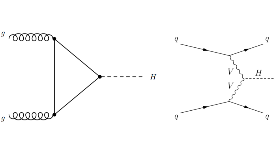
../_images/t03_higgsfeyn.png — Fig. 59 . Feynman diagrams for the gluon-gluon Fusion (ggF) process on the left and Vector Boson Fusion (VBF) on the right.
_{Image: ATLAS, CERN}#

The latter process, VBF, is very interesting to study as it probes the coupling between the Higgs boson and the two other vector bosons. This is seen on the Feynman diagram with the vertex between the two departing wavy branches of each vector boson V and the dashed line H representing the Higgs boson. Such configuration is said to be “sensitive to new physics”, because there can be processes that are not part of the current theory, the Standard Model, arising there. Hence the importance to measure the rates of VBF collisions (how frequent does it happen). But before, how to select the Higgs boson VBF production from the other one, gluon-gluon Fusion?

This is your mission!

Inside the Data#

This tutorial will use toy samples inspired by ATLAS Open Data, which makes proton–proton collision data from the LHC openly available for education.

In the VBF process, the initial quarks that first radiated the vector bosons are deflected only slightly and travel roughly along their initial directions. They are then detected as particle “jets” in the different hemispheres of the detector. Jets are reconstructed as objects. Although they are more of a conical shape, they are stored in the data as a four-vector entity, with a norm, two angles and an energy.

The collisions have been filtered to select those containing each a Higgs boson, four leptons^* and at least two jets.

We will focus on two variable for now:

\(|\Delta\eta_{jj}|\): it corresponds to the angle between the two jets (\(\eta\) is the pseudorapidity)
\(m_{jj}\): the invariant mass of the two jets

These variable are already calculated in the data samples.

Part I: Decision Stump By Hand#

1.1 Get the data#

Consider the three datasets:

lhc_atlas_higgs_train.csv lhc_atlas_higgs_valid.csv lhc_atlas_higgs_test.csv

For this tutorial, we will only need the training dataset.

Mount your Drive according to the Setup section, or retrieve it from your local folders if you are using Jupyter Notebook on your device.

Open a new Colaboratory and import the following:

import os, sys
import pandas as pd
import numpy as np

1.1.1 Explore#

Use pd.read_csv to store the dataset into a dataframe. Explore the variables by printing the first five rows.

The sample column stores the labels of the collisions: +1 corresponds to VFB and -1 to ggF.

Tasks:

How many events does the file contain?
How many events of each process (VBF and ggF) does the file contain?

Write down the proper commands for neat printing of your results.

1.1.2 Visualize the Training Data#

Let’s see a nice scatter plot of the training data, with \(|\Delta\eta_{jj}|\) on the \(x\)-axis and \(m_{jj}\) on the \(y\)-axis. The plotting macro is given in the Appendix: T3 Snippet Zone. Before using it, you will need to split your dataset into signal and background (if you have a look at the code snippet, you will understand why):

# Variables of interest
XNAME = 'detajj'; XLABEL = r'$|\Delta\eta_{jj}|$'
YNAME = 'massjj'; YLABEL = r'$m_{jj}$ (GeV)'

inputs = [XNAME, YNAME]

# Binning ranges
XBINS, XMIN, XMAX, XSTEP = 5, 0, 5, 1
YBINS, YMIN, YMAX, YSTEP = 5, 0, 1000, 200

# Split training data into signal and background
sig = ...
bkg = ...

Then pass sig and bkg to the plotting macro.

Hint

df.loc[rows, columns] lets you filter both rows and columns at the same time.

Call the macro and look at your data!

1.1.3 Prepare Dataset (Features & Labels)#

In this step, we will select the variables of interest (detajj and massjj) from the training dataset, and convert both the features and labels into NumPy arrays. Copy the following into your notebook and fill in the missing pieces (...):

# Extract detajj & massjj and convert to NumPy
X_train = ...
y_train = ...

1.2 Compute the Gini Index#

Recall the Gini’s index is defined as:

\[\begin{equation*} G_i = 1 - \sum_{k=1}^{N_\text{classes}} \left( \frac{N_{k, i}}{ N_i} \right)^2 \end{equation*}\]

Write a function computing the Gini index value. Make your code as general as possible. It should work for any array of labels and list of classes.

Bonus: Ensure your function handles empty nodes gracefully (i.e., avoid division by zero).

Use the following function signature:

def get_gini_index(y, classes):
    """
    y       : NumPy array of labels in the node
    classes : list of possible class values (e.g., [-1, 1])
    """

    # ... your code here... 

In the following cells, add a series of tests to make sure your function returns the correct answers.

1.3 Compute the Cost Function#

Write a simple function that returns the cost in relative impurity of dividing a node into two sub-nodes, defined as:

\[\begin{equation*} J(j, t_j) = \frac{N_\text{left}}{N_\text{node}} G_\text{left} + \frac{N_\text{right}}{N_\text{node}} G_\text{right} \;, \end{equation*}\]

where \(j\) is a given feature and \(t_j\) the associated threshold for that feature.

For now, we will not vectorize, so you can use this signature:

def get_cost(n_left, gini_left, n_right, gini_right):
    """
        ... write the docstring
    """

    # ... your code here

1.4 Decision Stump: Core of the Action#

Write the key function get_threshold_min_cost that will find the threshold on a given feature which minimizes the weighted Gini index, i.e., the value that maximizes the purity of the two resulting sub-nodes.

The function should return both the best threshold and the associated minimum cost. You can use the functions defined above (get_gini_index, get_cost) to help with the computation.

def get_threshold_min_cost(feature_values, y, classes, precision=0.01):
    """
    Find the threshold that minimizes the weighted Gini index.

    Parameters
    ----------
    ... 

    Returns
    -------
    ...

    """

    # ... your code here

Complete the docstring and write the function.

Hint 1

For a NumPy array a, you can select elements satisfying a condition using boolean indexing:
Example:

# Select values smaller than 5
indices = a < 5       # this creates a boolean array
selected_values = a[indices]

indices is a boolean array of the same shape as a.
selected_values contains the elements in a whose numerical value is less than 5.

Hint 2

A precision on the precision option 😉: It is the fraction of the feature range to use as step size for the threshold scanning. For example, precision=0.01 means thresholds will be tested every 1% of (max(feature) - min(feature)).

1.5 What Is the Best Split?#

Call get_threshold_min_cost on each of the two input features we are considering here. Conclude on the final cut for your decision stump.

1.6 Plot the Cut#

Adapt the plot_scatter macro so that it can also draw the decision boundary from the stump. You can use Matplotlib’s axhline or axvline methods for drawing a horizontal or vertical line respectively. Try to be as general as possible in the input arguments.

You just coded a decision stump by hand!

Part II: Smarter Threshold Search#

In Part I, we scanned all possible thresholds for each feature, counting left/right labels at every step. This brute-force approach has quadratic complexity with respect to the number of samples: for \(m\) samples, each threshold requires \(\mathcal{O}(m)\) operations, and there are roughly \(m\) thresholds, giving \(\mathcal{O}(m^2)\) per feature. That is, in total, \(\mathcal{O}(n m^2)\) for \(n\) features.

Can we do better? What about sorting each feature first?

You can have a look at Scikit-Learn’s DecisionTreeClassifier on the user guide, chapter Decision Trees to learn more about its efficient implementation.

Part III: Chain It Recursively: From Stump to Tree#

Now that you’ve coded a decision stump, how can you grow a full decision tree? Start by writing the pseudo-code first.

Decide on an exit condition: it could be reaching a maximum depth, a Gini index below a chosen threshold, or a minimum number of samples in a leaf.

Think about the output format: how will you record the sequence of splits in the feature space in a simple, readable way?

Have fun taking the best decisions and growing your tree!

Appendix: T3 Snippet Zone#

Scatter Plot#

To make titles, labels and legend entries big enough:

import matplotlib.pyplot as plt

FONTSIZE = 16
params = {
         'axes.labelsize': FONTSIZE,
         'axes.titlesize': FONTSIZE,
         'xtick.labelsize':FONTSIZE,
         'ytick.labelsize':FONTSIZE,
         'legend.fontsize':FONTSIZE}
plt.rcParams.update(params)

def plot_scatter(sig, bkg, 
              xname=XNAME, xlabel=XLABEL, xmin=XMIN, xmax=XMAX, xstep=XSTEP,
              yname=YNAME, ylabel=YLABEL, ymin=YMIN, ymax=YMAX, ystep=YSTEP,
              fgsize=(6, 6), ftsize=FONTSIZE, alpha=0.3, title="Scatter plot"):
  
  fig, ax = plt.subplots(figsize=fgsize)

  # Annotate x-axis
  ax.set_xlim(xmin, xmax)
  ax.set_xlabel(xlabel)
  ax.set_xticks(np.arange(xmin, xmax+xstep, xstep))

  # Annotate y-axis
  ax.set_ylim(ymin, ymax)
  ax.set_ylabel(ylabel)
  ax.set_yticks(np.arange(ymin, ymax+ystep, ystep))

  # Scatter signal and background:
  ax.scatter(sig[xname], sig[yname], marker='o', s=8, c='b', alpha=alpha, label='VBF')
  ax.scatter(bkg[xname], bkg[yname], marker='*', s=8, c='r', alpha=alpha, label='ggf')

  # Legend and plot:
  ax.legend(fontsize=ftsize, bbox_to_anchor=(1.04, 0.5), loc="center left", frameon=False) 
  ax.set_title(title, pad=20)
  plt.show()

Introduction
to Machine Learning

T3. Decision Stump

Contents

T3. Decision Stump#

Introduction#

Higgs boson production modes#

Inside the Data#

Part I: Decision Stump By Hand#

1.1 Get the data#

1.1.1 Explore#

1.1.2 Visualize the Training Data#

1.1.3 Prepare Dataset (Features & Labels)#

1.2 Compute the Gini Index#

1.3 Compute the Cost Function#

1.4 Decision Stump: Core of the Action#

1.5 What Is the Best Split?#

1.6 Plot the Cut#

Part II: Smarter Threshold Search#

Part III: Chain It Recursively: From Stump to Tree#

Appendix: T3 Snippet Zone#

Scatter Plot#

Introduction to Machine Learning

T3. Decision Stump

Contents

T3. Decision Stump#

Introduction#

Higgs boson production modes#

Inside the Data#

Part I: Decision Stump By Hand#

1.1 Get the data#

1.1.1 Explore#

1.1.2 Visualize the Training Data#

1.1.3 Prepare Dataset (Features & Labels)#

1.2 Compute the Gini Index#

1.3 Compute the Cost Function#

1.4 Decision Stump: Core of the Action#

1.5 What Is the Best Split?#

1.6 Plot the Cut#

Part II: Smarter Threshold Search#

Part III: Chain It Recursively: From Stump to Tree#

Appendix: T3 Snippet Zone#

Scatter Plot#

Introduction
to Machine Learning