Gradient Descent in Practice

How to choose a correct learning rate?

Short answer: inspect your gradient descent cost function.

Long answer:

Adjusting the learning rate

It is always a good programming practice to add in your code printouts, i.e. print() statements to inspect the current values of your variables. In gradient descent, it is advised to print the values of the parameters and the cost function after some iterations. Here is an example of printouts of simple linear regression showing the values of updated parameters \(\boldsymbol{\theta}\) every 10 epochs until \(N\) = 100, then every 100 epochs:

Starting gradient descent

Iter    0	θ₀ =  25.130	∂J/∂θ₀ =  -2.5948	θ₁ =   2.146	∂J/∂θ₁ = -42.9159	Cost = 56.84502
Iter   10	θ₀ =  23.260	∂J/∂θ₀ =   1.9969	θ₁ =   1.640	∂J/∂θ₁ =  -9.6267	Cost = 33.25208
Iter   20	θ₀ =  21.647	∂J/∂θ₀ =   2.7424	θ₁ =   1.711	∂J/∂θ₁ =  -2.4181	Cost = 27.31331
Iter   30	θ₀ =  20.205	∂J/∂θ₀ =   2.6824	θ₁ =   1.889	∂J/∂θ₁ =  -0.8322	Cost = 23.07411
Iter   40	θ₀ =  18.904	∂J/∂θ₀ =   2.4700	θ₁ =   2.075	∂J/∂θ₁ =  -0.4608	Cost = 19.63395
Iter   50	θ₀ =  17.729	∂J/∂θ₀ =   2.2437	θ₁ =   2.248	∂J/∂θ₁ =  -0.3540	Cost = 16.82019
Iter   60	θ₀ =  16.665	∂J/∂θ₀ =   2.0317	θ₁ =   2.406	∂J/∂θ₁ =  -0.3066	Cost = 14.51773
Iter   70	θ₀ =  15.703	∂J/∂θ₀ =   1.8383	θ₁ =   2.549	∂J/∂θ₁ =  -0.2745	Cost = 12.63362
Iter   80	θ₀ =  14.833	∂J/∂θ₀ =   1.6630	θ₁ =   2.678	∂J/∂θ₁ =  -0.2477	Cost = 11.09184
Iter   90	θ₀ =  14.045	∂J/∂θ₀ =   1.5044	θ₁ =   2.795	∂J/∂θ₁ =  -0.2239	Cost =  9.83019
Iter  100	θ₀ =  13.333	∂J/∂θ₀ =   1.3609	θ₁ =   2.901	∂J/∂θ₁ =  -0.2025	Cost =  8.79778
Iter  200	θ₀ =   9.058	∂J/∂θ₀ =   0.4993	θ₁ =   3.538	∂J/∂θ₁ =  -0.0743	Cost =  4.77406
Iter  300	θ₀ =   7.490	∂J/∂θ₀ =   0.1832	θ₁ =   3.771	∂J/∂θ₁ =  -0.0273	Cost =  4.23233
Iter  400	θ₀ =   6.914	∂J/∂θ₀ =   0.0672	θ₁ =   3.857	∂J/∂θ₁ =  -0.0100	Cost =  4.15940
Iter  500	θ₀ =   6.703	∂J/∂θ₀ =   0.0247	θ₁ =   3.888	∂J/∂θ₁ =  -0.0037	Cost =  4.14958
Iter  600	θ₀ =   6.625	∂J/∂θ₀ =   0.0091	θ₁ =   3.900	∂J/∂θ₁ =  -0.0013	Cost =  4.14825
Iter  700	θ₀ =   6.597	∂J/∂θ₀ =   0.0033	θ₁ =   3.904	∂J/∂θ₁ =  -0.0005	Cost =  4.14808
Iter  800	θ₀ =   6.587	∂J/∂θ₀ =   0.0012	θ₁ =   3.905	∂J/∂θ₁ =  -0.0002	Cost =  4.14805
Iter  900	θ₀ =   6.583	∂J/∂θ₀ =   0.0004	θ₁ =   3.906	∂J/∂θ₁ =  -0.0001	Cost =  4.14805


End of gradient descent after 1000 iterations

Picking a learning rate is a guess’n’check business.

Typical learning rates range between \(1\) and \(10^{-7}\). The common practice is to start with e.g. \(\alpha = 0.01\), a reasonable number of epochs, e.g. \(N = 100\) or \(1000\) (depending on the size of the data set), and see how the gradient descent behaves.

The cost function should decrease after every iteration. If the printouts show that the cost function and parameter are taking very, very large values: \(\alpha\) is too big, the gradient descent is diverging! One should reduce the learning rate by e.g. a factor 10 and see how the gradient behaves.

If the cost decreases after each iteration, this is a good sign that the gradient will converge. However it can converge very slowly if \(\alpha\) is too small, and as a consequence necessitate a large number of epoch before reaching the optimized parameter values. While tuning the hyperparameters, it is generally good to cap the number of epochs low and inspect the difference \(\Delta \theta = \theta^\text{new} - \theta^\text{prev}\) to see if the relative increment or decrement with respect to the \(\theta\) value is small. There is a bit of tweaking before finding a correct learning rate.

A graph to visualize the cost’s evolution

To inspect the gradient descent algorithm, it is convenient to store the intermediary values of the cost function and plot them with the iteration number on the \(x\) axis. The resulting curve should be strictly decreasing. Below is an example with different learning rates being plotted:

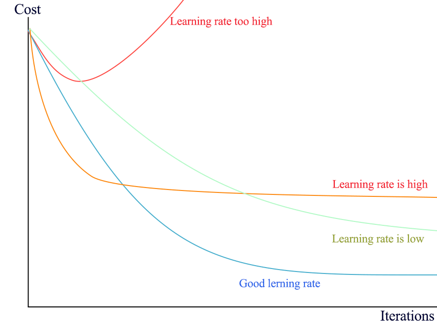
Fig. 9 : The learning rate plays a crucial role on the gradient’s speed towards convergence.
_{Credits: Jonathan Hui Medium}

Exercise

For each learning rate situation above, illustrate with a plot (qualitative drawing) the corresponding evolution of the model parameters.

Knowing when to stop

In mathematics, zero is exactly zero. In computing, variables can store very small numbers considered zero but with trailing non-zero digits. A good cutoff to declare the gradient descent algorithm successful is to exit when e.g. the cost function’s relative decrease is lower than a given threshold, for instance \(10^{-6}\).

Summary on Linear Regression

Key concepts

Linear Regression is the procedure that estimate a real-valued dependent variable (target) from independent variables (input features) assuming a linear relationship between \(n\) input features and \(n+1\) coefficients (parameters, or weight). The extra one is the offset parameter.

The cost function computes the sum of errors between the predicted line and the data. It usually uses the least squared method (errors squared).

The Gradient Descent is an optimization algorithm consisting of an iterative procedure to update the parameters in the direction of ‘descending gradient’, i.e. dictated by the slope of the cost function’s partial derivatives for each parameter, until convergence to values for the parameters minimizing the cost function.

Hyperparameters are quantitative entities controlling the learning algorithm.

The learning rate for gradient descent is an important hyperparameter that should be tuned to avoid divergence or over-shooting (learning rate too large) or slow convergence (learning rate too small) necessitating a high number of iterations (epochs).

 
The linear regression was our starting model. Nature and most dataset are far from being linear! Later in this course, we will see (slightly) more complex machine learning algorithms able to model non-linear behaviour. Linearity is an assumption that should be made with care.

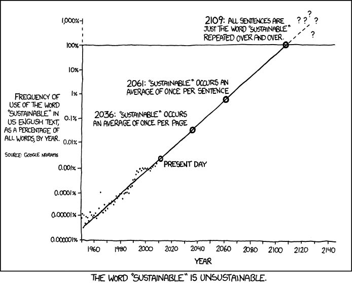
Fig. 10 : A questionable linear extrapolation, from the great webcomic xkcd.