Cost Function in Linear Regression
Contents
Cost Function in Linear Regression#
Definitions#
The accuracy of the mapping function is measured by using a cost function.
Definition 4
The cost function returns the global error between the predicted values from a mapping function \(h\) (predictions) and all the target values (observations) of the data set.
This is also called the average loss or empirical risk. The term empirical, meaning based on experience or experiment, indicates that this is a finite-sample average over the training dataset. Not an expectaction. The true risk, by contrast, is the expectation over the full data distribution, which is inaccessible because that distribution is unknown.
Let’s introduce the most popular cost function (over)used in machine learning:
Definition 5
The Mean Squared Error (MSE), also called squared error function is a commonly used cost function for linear regression. It is defined as:
You can recognize this expression as an average. In machine learning, an extra factor of \(\tfrac{1}{2}\) is sometimes included for convenience, since it cancels out when taking derivatives. In Equation (3), each \(h_\theta (x^{(i)})\) is a prediction done by our mapping function \(h_\theta\), whereas each \(y^{(i)}\) is an observed value in the data.
The initial goal to “fit the data well” can now be formulated in a mathematical way: find the parameters \(\theta_0\) and \(\theta_1\) that minimize the cost function:
Cooking with the Cost Function#
Now comes an exercise to compute the cost function ‘by hand’ so you can get a feel for the equation above… and, by a huge extrapolation, the staggering number of computations that happen in any machine learning task.
We’ll use a super simple dataset with just four samples:
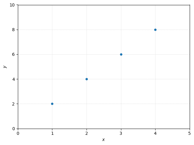
This is an ideal case for pedagogical purposes. What are the values of \(\theta_0\) and \(\theta_1\) here?
Check your answers
Recall the mapping function for linear regression: \(h_\theta(x) = \theta_0 + \theta_1 x\). As we have a correspondance \(y = 2x\) for all points, so \(h_\theta(x) = 2x\), so \(\theta_0 = 0\) and \(\theta_1 = 2\).
You will appreciate the simplification, as we will calculate the cost by hand for different values of \(\theta_1\). More complicated things await you in the tutorial, promised.
Exercise
We will set our intercept term to its optimized value: \(\theta_0\) = 0 and vary only the slope, that is \(\theta_1\).
Start with a value of \(\theta_1\) = 1 and calculate the cost function \(C(\theta_1)\).
Proceed the same for other values of \(\theta_1\) of 0.5, 1.5, 2, 2.5, 3.
How would the graph of the cost function \(C(\theta_1)\) as a function of \(\theta_1\) look like?
Are there maxima/minima? If yes how many?
Solutions ✋ Don’t look too soon! Give it a try first.
The values of the cost function for each \(\theta_1\) are reported on the plot below:
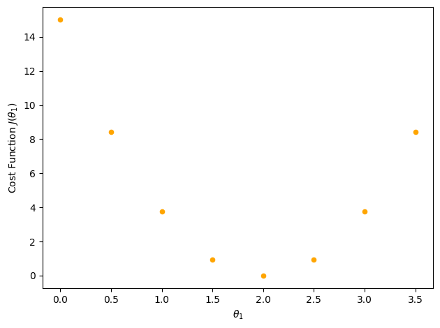
We see that in this configuration, as we ‘swipe’ over the data points with ‘candidate’ straight lines, there will be a value for which we minimize our cost function. That is the value we look for (but you will learn to make such fancy plot during the tutorials).
This was with only one parameter. How do we proceed to minimize with two parameters?
Visualizing the cost#
Let’s see a visual representation of our cost function as a function of our \(\theta\) parameters. We saw in the simple example above that the cost function \(C(\theta_1)\) with only one parameter is a U-shaped parabola. The same goes if we fix \(\theta_1\) and vary \(\theta_0\). Combining the two, it will look like a bowl. The figure below is not made from the data above, just for illustration:
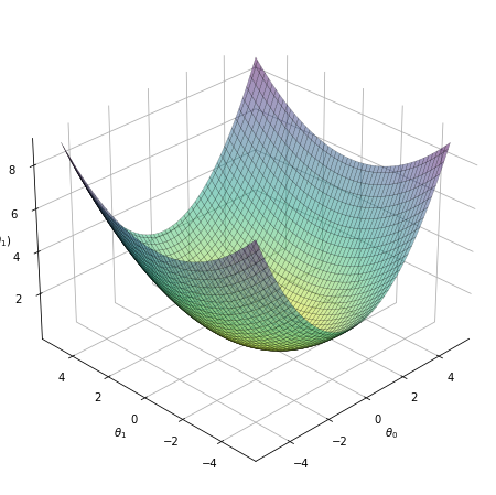
Fig. 2 . The cost function (vertical axis) as a function of the parameters \(\theta_0\) and \(\theta_1\).#
What does this represent? It shows the result of the cost function calculated for a range of \(\theta_0\) and \(\theta_1\) parameters. For each coordinate (\(\theta_0\) , \(\theta_1\)), there has been a loop over all the training data set to get the global error. The vertical value shows thus how ‘costly’ it is to pick up a given (\(\theta_0\) , \(\theta_1\)). The higher, the worse is the fit. The center of the bowl, where \(C(\theta_0 , \theta_1)\) is minimum, corresponds to the best choice of the \(\theta\) parameters. In other words: the best fit to the data.
How do we proceed to find the \(\theta_0\) and \(\theta_1\) parameters minimizing the cost function?