Performance Metrics
Contents
Performance Metrics#
In supervised learning, assessing a model’s performance is about how close predictions are to the truth. Before digging into the metrics, let’s first define the types of errors properly.
Types of errors#
Generally speaking, an error is the gap between the prediction and the true value. There are different terms depending on the algorithm and the set on which errors are computed.
For regression algorithms#
Definition 25
A residual is the difference between the actual and predicted value computed with respect to data samples used to train, validate and tune the model.
\(\rightarrow\) in-sample error
It is always a good practice to make a scatter plot of all the residuals with respect to the independent variable values; they should be randomly distributed on a band symmetrically centered at zero. If not, this means the chosen model is not appropriate to correctly fit the data.
Definition 26
The generalized error is the difference between the actual and predicted values, averaged over test or new data samples.
\(\rightarrow\) out-of-sample error
For classification algorithms#
In classification, the errors bear different names. As we saw that multiclassifiers are treated as a collection of binary classifiers, we will go over the two types of errors.
Recall that the labelling and numerical association (1 and 0) of classes is arbitrary. Signal can be the rare process we want to see in the detector and 0 the background we want to reject. But we could exchange the numbers with 0 and 1, provided we remain consistent. In medical diagnosis, the class labelled 1 can be the presence of cancer on a patient (it’s not what we want of course, but what we are looking to classify).
Definition 27
The confusion matrix is a table used to visualize the prediction results (positive/negative) from a classification algorithm with respect to their correctness (true/false).
It is a \(n^C \times n^C\) matrix, with \(n^C\) the number of classes.
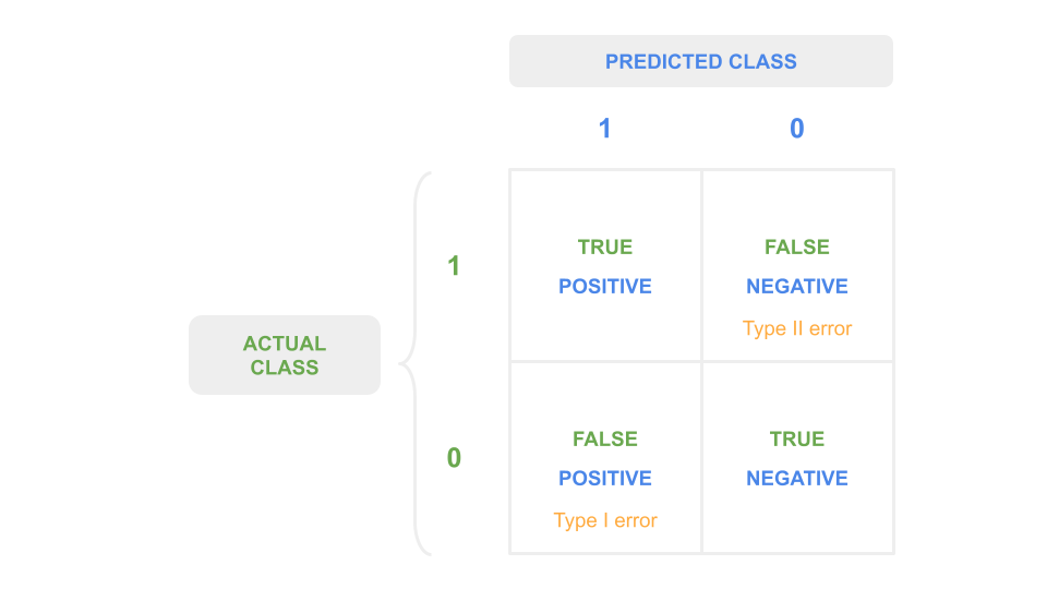
Fig. 16 : The confusion matrix for a binary classifier.
Image from the author#
The quantity in each cell \(C_{i,j}\) corresponds to the number of observations known to be in group \(i\) and predicted to be in group \(j\). The true cells are along the diagonal when \(i=j\). Otherwise, if \(i \neq j\), it is false. For \(n^C =2\) there are two ways to be right, two ways to be wrong. The counts are called:
\(C_{0,0}\): true negatives
\(C_{1,1}\): true positives
\(C_{0,1}\): false positives
\(C_{1,0}\): false negatives
Here is a rephrase in the context of event classification: signal (1) versus background (0).
True positives
We predict signal and the event is signal.
True negatives
We predict background and the event is background.
False positives
We predict signal but the event is background: our signal samples will have background contamination.
False negatives
We predict background but the event is signal: we have signal contamination in the background but most importantly: we missed a signal event!
The false positive and false negative misclassifications are also referred to as type I and type II errors respectively. They are usually phrased using statistical jargon of null hypothesis (background) and alternative hypothesis (signal). The definitions below merge the statistical phrasing with our context above:
Definition 28
Type I error - False Positive
Error of rejecting the null hypothesis when the null hypothesis is true.
👉 Background is classified as signal (background contamination)
Type II error - False Negative
Error of accepting the null hypothesis when the alternative one is actually true.
👉 Signal is classified as background (missing out on what we look for)
The type I error leads to signal samples not pure, as contaminated with background. But a type II error is a miss on a possible discovery! Or in medical diagnosis, it can be equivalent to state “you are not ill” to a sick patient. Type II errors are in some cases and contexts much worse than type I errors.
Performance measures#
For regression algorithms#
There are many metrics used to evaluate the performance of regression algorithms, each with their pros and cons.
The most common metric is the root mean squared error (RMSE).
Definition 29
The root mean squared error (RMSE) is the square root of the mean squared error:
RMSE ranges from 0 to infinity. The lower the RMSE, the better. By taking the square root we have an error of the same unit as the target variable \(y\) we want to predict.
You may have seen in a statistics course the coefficient of determination, called \(R^2\) or \(r^2\). This is not really a measure of model performance, although it can be used as a proxy. What \(r^2\) does is to measure the amount of variance explained by the model. It is more of a detector of variance than a performance assessment. Ranging from 0 to 1, with 1 being ideal.
For classification algorithms#
The more popular error measurements associated with machine learning are defined below:
Definition 30
Accuracy
Measures the fraction of correct predictions among all predictions
Precision, or Positive Predictive Value (PPV)
Measures the fraction of true positive predictions among all positive predictions.
Recall, or True Positive Rate (TPR)
Measures the fraction of true positive predictions among all true observations.
F-Score, or F1
Describes the balance between Precision and Recall. It is the harmonic mean of the two:
The accuracy has the limitation of mixing types I and II errors: it may not reflect the model performance on minority classes in case of an unbalanced dataset. The Precision and Recall allow evaluation that distinguishes between false positives and false negatives.
The F-Score is a single metric favouring classifiers with similar Precision and Recall. But in some contexts, it is preferable to favour a model with either high precision and low recall, or vice versa. There is a known trade-off between precision and recall.
Case of unbalanced dataset
In an unbalanced dataset, some classes will appear much more frequently than others. A specific metric called balanced accuracy is used to assess the performance in that case.
Definition 31
Balanced accuracy is calculated as the average of recalls obtained on each class.
Exercise
Find different examples of classification in which:
a low recall but high precision is preferable
a low precision but high recall is preferable