T2. Classifier

In this tutorial, you learn step by step how to code a binary classifier by hand!

Don’t worry, the process will be guided.

Learning Objectives

• Retrieve and pre-process a dataset for binary classification

• Implement logistic regression in Python

• Plot training and testing costs against iterations

• Compute performance metrics and verify them with standard libraries

• [Bonus] From the model parameters, derive the equations of straight lines representing different decision boundaries, and draw them on a scatter plot

Introduction: calorimeter showers

A calorimeter in the context of experimental particle physics is a sub-detector aiming at measuring the energy of incoming particles. At CERN Large Hadron Collider, the giant multipurpose detectors ATLAS and CMS are both equipped with electromagnetic and hadronic calorimeters. The electronic calorimeter, as its name indicates, is measuring the energy of incoming electrons. It is a destructive method: the energetic electron entering the calorimeter will interact with its dense material via the electromagnetic force. It eventually results in the generation of a shower of particles (electromagnetic shower), with a characteristic average depth and width. The depth is along the direction of the incoming particle and the width is the dimension perpendicular to it.

Problem? There can be noisy signals in electromagnetic calorimeters that are generated by hadrons, not electrons.

Your mission is to help physicists by coding a classifier to select electron-showers (signal) from hadron-showers (background).

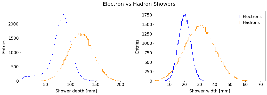
To this end, you are given a dataset of shower characterists from previous measurements where the incoming particle was known. The main features are the depth and the width.

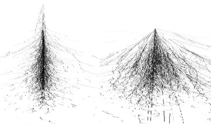
Fig. 57 Visualization of an electron shower (left) and hadron shower (right).
_{From ResearchGate}

Hadron showers are on average longer in the direction of the incoming hadron (depth) and large in the transverse direction (width).

Part I: Linear Classifier By Hand (Guided)

1.1 Get the data

Download dataset

Mount your Drive according to the Setup section, or retrieve it from your local folders if you are using Jupyter Notebook on your device.

Open a new Colaboratory and import the following:

import sys, os
import numpy as np
import pandas as pd

1.2 Data pre-processing

1.2.1 Explore the Data

Read the dataset into a dataframe df. What are the columns? Which column stores the labels (targets)? How many samples are there?

1.2.2 Labels to Binary

The target column contains alphabetical labels. Create an extra column in your dataframe called y containing 1 if the sample is an electron shower and 0 if it is a hadron one.

Hint: you can first create an extra column full of 0, then apply a filter using the .loc property from DataFrame. It can be in the form:

df.loc[ CONDITION, COLUMN_TO_UPDATE] = VALUE

Read the pandas documentation on .loc.

1.2.3 Create Feature Matrix \(X\)

Select the input feature columns and create the feature matrix \(X\) of shape \((m, n)\), and extract the target vector \(y\) of shape \((m,)\). Call the method .to_numpy() like you did in Tutorial 1. Check if you have the correct shapes:

X = ... 
y = ... 

# Check shapes
print("X shape:", X.shape)
print("y shape:", y.shape)

1.2.4 Train/Test Split

Split the dataset into training and testing sets using 80/20 proportion. For this, copy paste the following in your code:

from sklearn.model_selection import train_test_split

X_train, X_test, y_train, y_test = train_test_split(
    X, y, test_size=0.2, random_state=42
)

# Check shapes
print(f"X_train: {X_train.shape}, y_train: {y_train.shape}")
print(f"X_test:  {X_test.shape},  y_test: {y_test.shape}")

Do the shape make sense?

1.2.5 Feature Scaling

Let’s scale our input features using the standardization method. Which dataset(s) should be scaled and why?

# Get mean and std from training data
mean_train = ...
std_train = ...

# Standardize training
X_train_scaled = ...

# Standardize test data
X_test_scaled  = ...

# Check
print("X_train_scaled mean:", X_train_scaled.mean(axis=0))
print("X_train_scaled std:", X_train_scaled.std(axis=0))

1.2.6 Feature Matrix Augmentation

We will add a column of ones to our matrix \(X\) to simplify the vectorized computations with the bias term (\(\theta_0\) in our notations). For this, use NumPy’s hstack method:

X_train_aug = np.hstack(...)
X_test_aug  = np.hstack(...)

Try to predict the resulting shapes first, then check them and see if they make sense.

1.3 Functions

Important

Test your functions with small dummy arrays to ensure correct outputs.

We saw a lot of functions in the lectures: hypothesis, logistic, cost, etc. We will code these functions in Python to make the code more modular and easier to read.

Warning

In the following you will work with two dimensional NumPy arrays. Make sure the objects you declare in the code have the correct dimension (number of rows and number of columns).

1.3.1 Hypothesis Function

^* docstring, short for “documentation string,” is a commented paragraph of code at the top of a file or of the definition of a function. It explains the arguments, their types, what the function should return, etc. Think of it as a mini manual. Writing docstring is a common practice to make code readable.

Write a function computing the linear sum of the features \(X\) with the \(\boldsymbol{\theta}\) parameters for each input sample. Caution here: \(X\) is the augmented matrix of input features. To help you, the docstring^* is provided:

def lin_sum(X, thetas):
    """
    Compute the linear combination of input features and parameters.

    Parameters
    ----------
    X : array-like, shape (m_samples, n_features+1)
        Input features (already augmented with a column of ones for bias).
    thetas : array-like, shape (n_features+1,)
        Parameter vector including bias term.

    Returns
    -------
    ndarray, shape (m_samples, 1)
        Linear sum for each sample.
    """

    # Your code here

What should be the dimensions of the returned object? Make sure your function returns a 2D array with the correct shape.

1.3.2 Logistic Function

Write a function computing the logistic function:

 def sigmoid(z):

    # Your code here 

Be careful to call the correct library so that your function works with arrays both as inputs and outputs.

1.3.3 Partial Derivatives of Cross-Entropy Cost Function

In the linear assumption, the partial derivatives of the cross-entropy cost function are (amazingly) the same as with the Mean Square Error:

\[\frac{\partial}{\partial \theta_j} \text{Cost}(\boldsymbol{\theta}) = \frac{1}{m} \sum_{i=1}^{m} \left( h_\theta(x^{(i)}) - y^{(i)}\right) x_j^{(i)}\]

Write a function that computes the gradient vector for all features at once. The provided docstring should help you translate the mathematical formulation into clean, vectorized code.

def gradient_cross_entropy(y_true, y_pred, X):
    """
    Compute the gradient vector of the cross-entropy cost function.

    Parameters
    ----------
    y_true : array-like, shape (m,) or (m,1)
        Binary target (0 or 1) for each sample.
    y_pred : array-like, shape (m,) or (m,1)
        Predicted score for each sample.
    X : array-like, shape (m, n_features+1)
        Input features, already augmented with a column of ones for bias.

    Returns
    -------
    ndarray, shape (n_features+1, 1)
        Column vector of partial derivatives with respect to each model parameter.
    """

    # Your code here

You can use reshape(-1, 1) on the relevant variable(s) to ensure they have the correct dimension.

The output is the vector of partial derivatives with respect to each parameter (\(\theta_j\) in our notations). Remember to test your function with small dummy arrays of the correct shape!

1.3.4 Cross-Entropy Cost Function

Write a function computing the total cost from the vectors of predicted and true values. Reminder of the cross-entropy cost:

\[C(\boldsymbol{\theta}) = - \frac{1}{m} \sum_{i=1}^{m} \Big[ y^{(i)} \log(h_\theta(x^{(i)})) + (1 - y^{(i)}) \log(1 - h_\theta(x^{(i)})) \Big]\]

def cross_entropy_cost(y_true, y_pred):

    # Your code here

A hint

You should use np.log, which computes the natural logarithm (base e).

A good trick

For numerical stability, you can clip your vector of scores y_pred to a small range, e.g.

y_pred = np.clip(y_pred, 1e-15, 1 - 1e-15)

This prevents taking \(\log(0)\).

Why clip values close to 1 as well? Look at the cross-entropy cost: you’ll see why clipping on both ends is necessary.

1.4 Classifier Loop

The core of the action.

Luckily a skeleton is provided. You will have to replace the statments # ... by proper code. It will mostly consist of calling the functions you defined in the previous section.

Test your code frequently. To do so, you can assign dummy temporary values for the variables you do not use yet, so that python knows they are defined and your code can run.

You can use again the should_print_iteration from the Snippet Zone sub-section Pretty Printing in Tutorial 1.

Subtlety with 2D arrays

You may compute some dot products resulting in a scalar. With 2D arrays, the single component of a “scalar” (1,1) NumPy array is still treated as a 2D array, and Python cannot access its value directly. To retrieve the actual number — for example, for printing — you need to call .item(), e.g. my_1_x_1_array2d.item().

Note on Exit Conditions

We saw earlier that we ought to stop the gradient descent loop if the partial derivatives of the cost get close to zero. This can be implemented by checking the norm of the gradient and stopping once this magnitude (always positive, by construction) falls below a predefined threshold. This provides a good measure of convergence.

However, the cost function may continue to decrease even when the gradients are small, potentially missing a better local minimum. To address this, you can perform another check at the end of each loop: stop when the change in cost between iterations drops below a threshold, for example:

if abs(cost_train_current_iteration - cost_previous_iteration) < 1e-8:

This is just an example; you’ll need to adapt it to your own variables and, instead of hardcoding the value, define a tolerance parameter (e.g. cost_tol) before starting the loop. Such a condition is less sensitive to feature scaling and ensures you don’t stop too early just because the gradient is small while the cost is still decreasing.

You can implement this dual stopping criterion:

• gradient norm

• cost change and observe the effect on convergence.

# Hyperparameters
alpha       = ...    # learning rate
N           = ...    # maximum number of iterations
epsilon     = 1e-6   # tolerance threshold for gradient norm (stopping criterion)
cost_tol    = 1e-8   # tolerance threshold for cost drop (stop. criterion)
cost_change = np.inf # initialize cost change for first iteration

# Number of features + 1 (number of columns in X)
n_param = ...

# Initialization of theta vector
thetas = ...

# Storing cost values for train and test datasets
costs_train = []
costs_test  = []

print("Starting gradient descent\n")

# -------------------
#   Start iterations
# -------------------
for iter_idx in range(N):
    # Get predictions (hypothesis function)
    # ... your code here ...

    # Calculate and store costs with train and test datasets
    cost_train = cross_entropy_cost(y_train, y_pred_train)
    cost_test  = cross_entropy_cost(y_test, y_pred_test)
    costs_train.append(cost_train)
    costs_test.append(cost_test)

    # ... your code here for gradient computation & parameter update


    # Cost change (for early stopping & printing)
    if iter_idx > 0:
        cost_change = cost_train - costs_train[-2]

    # Print selected iterations
    if should_print_iteration(iter_idx, 10, 100, 100):
        print(
            f"Iter {iter_idx:>4}\t"
            f"‖grad‖ = {grad_cost_norm.item():.4e}\t"
            f"Train cost = {cost_train:.5e}\t"
            f"Cost change = {cost_change:>+10.2e}\t"
            f"Test cost = {cost_test:.5e}"
        )

    # Exit conditions
    # ... your code here ...

print(f'\nEnd of gradient descent after {iter_idx+1} iterations')

print('Optimized parameters:')
for j in range(len(thetas)):
    print(f'\tParameter {j} = {thetas[j,0]:.4f}')

If you’re stuck, call the instructor or the teaching assistants and we will be happy to help you.

1.5 Plot cost versus epochs

Use the macro given in the section Plotting Macro: Cost vs Iteration from the Appendix: T2 Snippet Zone below to plot the variation of the total cost vs the iteration number. Call this macro:

plot_cost_vs_iter(costs_train, costs_test)

You should get something like this:

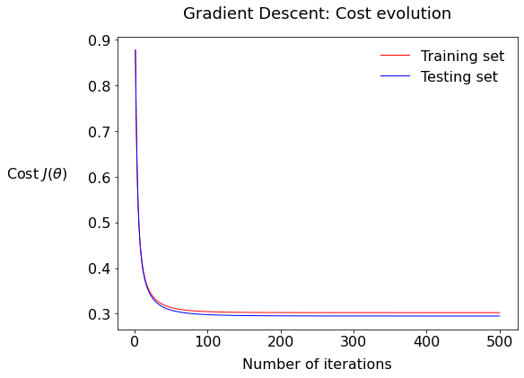
1.5.1 Plot Interpretation

Describe the plot; what is the fundamental difference between the two series train and test?

1.5.2 Cost gap?

What would it mean if there were a larger gap between the training and test cost values?

1.6 Performance Measures

We will write our own functions to quantitatively assess the performance of the classifier.

1.6.1 Binary Predictions

Before counting the true and false predictions, we need… predictions! So far, we have written functions that output a continuous value between 0 and 1, which can be interpreted as a probability. The function below converts these values into binary predictions (0 or 1). For the decision boundary, we will use 0.5 for now. Copy this to your notebook:

def make_predictions(thetas, X, boundary=0.5):
    scores = sigmoid(lin_sum(X, thetas)).flatten() # shape (m,)
    return (scores >= boundary).astype(int)

Your task here: try to write a nice docstring for this function.

Now we are ready to compute some performance metrics!

1.6.2 Accuracy

Write a function to compute the classifier’s accuracy manually. By “manually” we mean: explicitly compute the numerator and denominator. It’s more about coding pedagogically than efficiently, so as to improve your understanding.

1.6.3 Recall

Do the same for the recall. Compute it step by step, and then compare your results with those of your peers!

Part II: Draw Decision Boundaries

By drawing a decision boundary, you will grasp how the hypothesis formulation translates into a graphical separation in the feature space. We will work out the math behind this parametrization.

The goal
We want to draw on a scatter plot of the input features the lines corresponding to different decision boundaries.

Tip

Scroll down at the very end to see where we are heading to.

2.1 Scatter plot

The first step is to split the signal and background into two different dataframes. Using the general dataframe df defined at the beginning:

all_sig = df[df['type'] == 'electron'][['shower_depth', 'shower_width']]
all_bkg = df[df['type'] ==  'hadron' ][['shower_depth', 'shower_width']]

Then use the plotting macro in Scatter Plot (Part II) from the Appendix: T2 Snippet Zone to see a nice scatter plot. To call it:

plot_scatter(all_sig, all_bkg,
             figsize=(6, 6), fontsize=20, alpha=0.2, title="Calorimeter Showers")

2.2 Useful Functions

Recall the logistic function:

\[\hat{y} = \frac{1}{1 + e^{-z}}\]

Write a function rev_sigmoid that outputs the value \(z = f(\hat{y})\).

Write a function scale_inputs that scales a list of raw input features, either \(x_1\) or \(x_2\), according to the standardization procedure.

Write the function unscale_inputs that does the contrary.

2.3 Boundary Line Coordinates

2.3.1 Line Equation

For a given threshold \(\hat{y}\), write the equation of the line boundary: \(x_2 = f(\boldsymbol{\theta}, x_1, \widehat{y})\).

2.3.2 Coordinate points

To draw a line on a plot in Matplotlib, one needs to provide the coordinates as a set of two data points.

Write a function that compute the coordinates x2_left and x2_right – associated with the values of x1_min and x1_max respectively – of a decision boundary line at a given threshold \(\hat{y}\). (recall 0.5 is the standard one for logistic regression).

def get_boundary_line_x2(thresholds, thetas, 
                         x1min=X1MIN, x1max=X1MAX,
                         train_mean=MEAN_TRAIN, train_std=STD_TRAIN):
  # Your code here

Extra challenge? Compute this for several thresholds, i.e. the function returns a list of line coordinates for each thresholds.

Tip

It’s convenient to store the result in a dictionary. For instance you can have keys threshold, x2_left, x2_right.

2.4 Let’s Plot the Boundary

In the scatter plot code provided, uncomment the boundary section and draw the line(s) using the Matplotlib plot function. It will have this form:

   #... 
   ax.plot([x1min, x1max], [x2_left, x2_right], color='r', ls='-', lw=2)
   #... 

In the very end, this is how it would render:

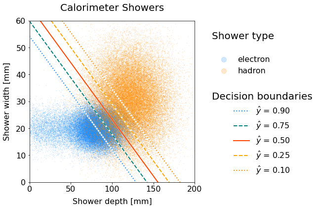
Fig. 58 Scatter plot of electron and hadron showers with decision boundary lines for various thresholds.

The higher the threshold, the more the boundary line shifts downwards in the electron-dense area. Why is that the case?

Part III: OOP

Turn your classifier into a class!

This is less guided, yet can be done in groups with an OOP-Jedi.

Tips

• Give it a try without any assistance first, just listing the attributes and methods.

• For scaling the features, a separate class FeatureScaler can be handy.

Appendix: T2 Snippet Zone

Plotting Macro: Cost vs Iteration

def plot_cost_vs_iter(train_costs, test_costs, title="Gradient Descent: Cost evolution"):
  
  fig, ax = plt.subplots(figsize=(8, 6))

  iters = np.arange(1,len(train_costs)+1)

  ax.plot(iters, train_costs, color='red', lw=1, label='Training set')
  ax.plot(iters, test_costs, color='blue', lw=1, label='Testing set')

  ax.set_xlabel("Number of iterations")
  ax.set_ylabel(r"Cost $J(\theta)$", rotation="horizontal")
  ax.yaxis.set_label_coords(-0.2, 0.5)

  ax.legend(loc="upper right", frameon=False)
  ax.set_title(title, fontsize=18, pad=20)
  plt.show()

Scatter Plot (Part II)

X1NAME = 'shower_depth'; X1LABEL = 'Shower depth [mm]'
X2NAME = 'shower_width'; X2LABEL = 'Shower width [mm]'
X1MIN  = 0 ; X1MAX = 200 
X2MIN  = 0 ; X2MAX =  60 

# Raw scatter plot
def plot_scatter(sig, bkg, boundaries=False,
                 x1name=X1NAME, x1label=X1LABEL, x1min=X1MIN, x1max=X1MAX,
                 x2name=X2NAME, x2label=X2LABEL, x2min=X2MIN, x2max=X2MAX,
                 figsize=(6, 6), fontsize=20, alpha=0.2, title="Scatter plot"):

  fig, ax = plt.subplots(figsize=figsize)

  # ------------------
  #      A X E S  
  # ------------------
  ax.set(xlim=(x1min, x1max), ylim=(x2min, x2max))
  ax.set_xlabel(x1label); ax.set_ylabel(x2label)

  # ------------------
  #   S C A T T E R   
  # ------------------
  scat_el = ax.scatter(sig[x1name], sig[x2name], marker='.', s=1, c='dodgerblue', alpha=alpha)
  scat_had= ax.scatter(bkg[x1name], bkg[x2name], marker='.', s=1, c='darkorange', alpha=alpha)
  
  # ----------------------
  #  B O U N D A R I E S
  # ----------------------
  # if boundaries: 
    # ... your code here ...

  # ------------------
  #   L E G E N D S 
  # ------------------
  # Legend scatter
  h = [scat_el, scat_had]
  legScatter = ax.legend(handles=h, labels=['electron', 'hadron'],
                         title="Shower type\n", title_fontsize=fontsize, markerscale=20,
                         bbox_to_anchor=(1.06, 0.8), loc="center left" , frameon=False)
  
  # Legend boundary
  if boundaries:
    ax.add_artist(legScatter)
    legLines = ax.legend(title="Decision boundaries", 
                       bbox_to_anchor=(1.06, 0.3), loc="center left", 
                       title_fontsize=fontsize, frameon=False)

  ax.set_title(title, fontsize=fontsize, pad=20)
  print('\n\n') ; plt.show()