Cost Function for Classification

Wavy least squares

If we plug our sigmoid hypothesis function \(h_\boldsymbol{\theta}(x)\) into the cost function defined for linear regression (Equation (3) from Lecture Cost Function for Linear Regression), we will have a complex non-linear function that could be non-convex.

Refresher on convex functions

A convex function has at least one global minimum, and if it is strictly convex, the minimum is unique.

Mathematically:
A function \(f: \mathbb{R}^n \to \mathbb{R}\) is convex if, for all \(x_1, x_2 \in \mathbb{R}^n\) and for all \(\lambda \in [0,1]\), we have:

(18)\[f\big(\lambda x_1 + (1-\lambda) x_2\big) \leq \lambda f(x_1) + (1-\lambda) f(x_2).\]

Intuitively: a straight line between any two points on the graph of the function lies above the graph itself.

In other words, the function “curves upwards” or is “bowl-shaped.”

Consider this function:

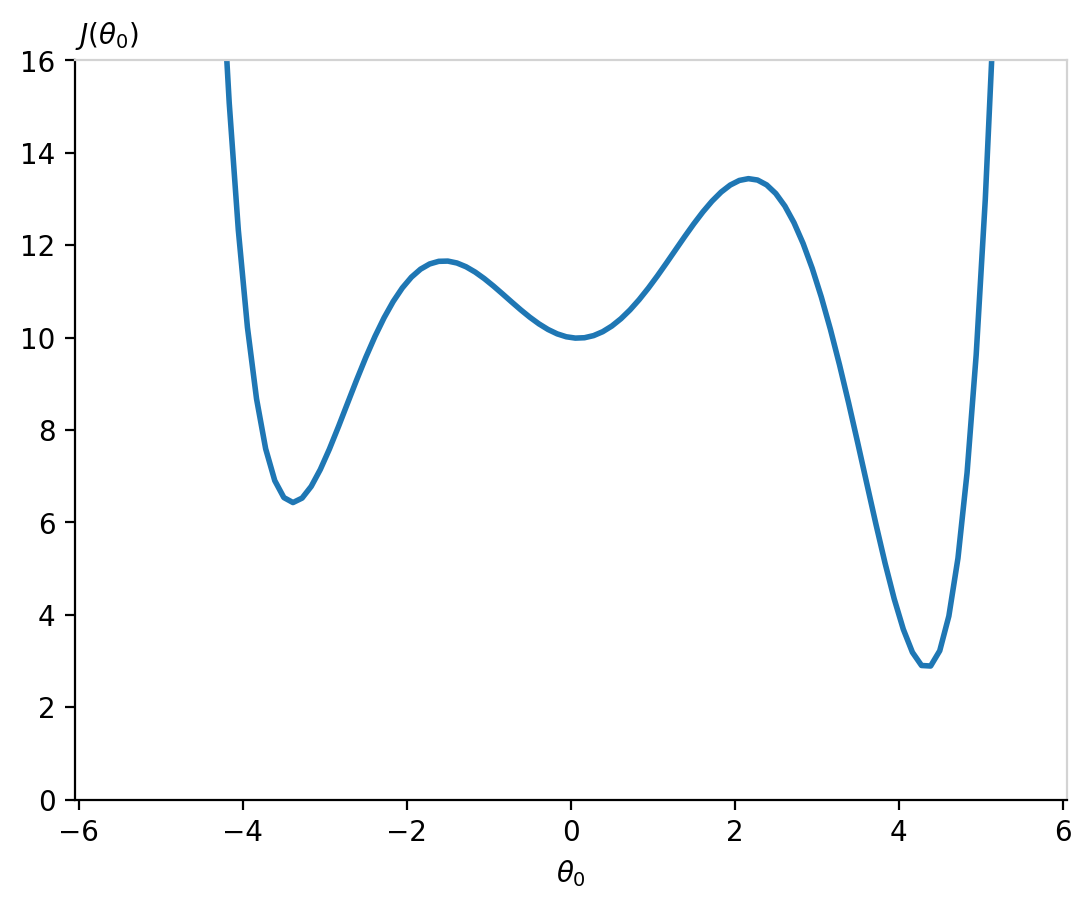
Imagine running a gradient descent procedue that starts from a randomly initialized \(\theta_0\) parameter around zero (or worse, lower than -2). It will fall into a local minima. Our cost function will not be at the global minimum! It is crucial to work with a cost function accepting one unique minimum.

Building a new cost function

As we saw in the previous section, the sigmoid fits the 1D data distribution very well. Our cost function will use the hypothesis \(h_\boldsymbol{\theta}(\boldsymbol{x})\) function as input. Recall that the hypothesis \(h_\boldsymbol{\theta}(\boldsymbol{x})\) is bounded between 0 and 1. What we need is a cost function producing high values if we mis-classify events and values close to zero if we correctly label the data. Let’s examine what we want for the two cases:

Case of a signal event:
A data point labelled signal verifies by our convention \(y=1\). If our hypothesis \(y^\text{pred} = h_\boldsymbol{\theta}(\boldsymbol{x})\) is also 1, then we have a good prediction. The cost value should be zero. If however our signal sample has a wrong prediction \(y^\text{pred} = h_\boldsymbol{\theta}(\boldsymbol{x}) = 0\), then the cost function should take large values to penalize this bad prediction. We need thus a strictly decreasing function, starting with high values and cancelling at the coordinate (1, 0).

Case of a background event:
The sigmoid can be interpreted as a probability for a sample being signal or not (but note it is not a probability distribution function). As we have only two outcomes, the probability for a data point to be non-signal will be in the form of \(1 - h_\boldsymbol{\theta}(\boldsymbol{x})\). We want to find a function with this time a zero cost if the prediction \(y^\text{pred} = h_\boldsymbol{\theta}(\boldsymbol{x}) = 0\) and a high cost for an erroneous prediction \(y^\text{pred} = h_\boldsymbol{\theta}(\boldsymbol{x}) = 1\).

Now let’s have a look at these two functions:

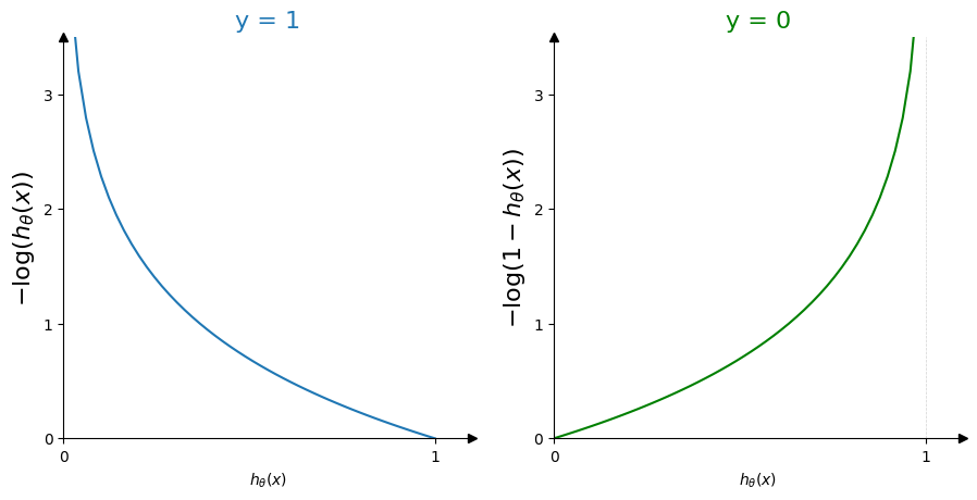
For each case, the cost function has only one minimum and harshly penalizes wrong prediction by blowing up at infinity.
How to combine these two into one cost function for logistic regression?
Like this:

Definition 18

The cost function for logistic regression is defined as:

(19)\[C(\boldsymbol{\theta}) = - \frac{1}{m} \sum^m_{i=1} \left[ \;\; {\color{RoyalBlue}y^{(i)} \log\left( h_\boldsymbol{\theta}(\boldsymbol{x}^{(i)} ) \right) }\;\;+\;\; {\color{OliveGreen}(1- y^{(i)}) \log\left( 1 - h_\boldsymbol{\theta}(\boldsymbol{x}^{(i)} ) \right)} \;\;\right]\]

This function is also called cross-entropy loss function and is the standard cost function for binary classifiers.

Note the negative sign factorized at the beginning of the equation. The first and second term inside the sum are multiplied by \({\color{RoyalBlue}y^{(i)}}\) and \({\color{OliveGreen}(1 - y^{(i)})}\). This acts as a “switch” between the two possible cases for the targets: \({\color{RoyalBlue}y=1}\) and \({\color{OliveGreen}y=0}\). If \({\color{RoyalBlue}y=1}\), the second term cancels out and the cost takes the value of the first. If \({\color{OliveGreen}y=0}\), the first term vanishes. The two mutually exclusive cases are combined into one mathematical expression.

Generalization for \(K\) classes

The cross-entropy cost function we defined for binary classification can be naturally extended to handle \(K\) classes.

Notations

Recall the notations we use in binary classification. From an input vector \(\boldsymbol{x} = (x_1, \cdots , x_n)\) of \(n\) input features, we combine it with \(n+1\) model parameters \(\boldsymbol{\theta} = (\theta_0, \theta_1, \cdots, \theta_n)\) linearly:

(20)\[z^{(i)} = \sum_{j=1}^{n_\text{features}} \theta_{j} x_j^{(i)} = \boldsymbol{\theta}^\top \boldsymbol{x}^{(i)}\]

In the following, we will write \(\hat{y}\) instead of \(y^\text{pred}\) to lighten the equations. Both refers to a prediction.

So the pipeline for binary classification is:

(21)\[\boldsymbol{x}^{(i)} \xrightarrow{ \text{linear map }\;\boldsymbol{\theta}^\top \boldsymbol{x}^{(i)}\;} z^{(i)} \xrightarrow{\;\text{logistic function }\sigma(z^{(i)})\;} \hat{y}^{(i)}\]

At the end, the target for a given sample \(i\) is one value (a scalar).

But now we have \(K\) classes. The prediction is no longer one value but our hypothesis should output a \(K\)-dimensional vector. As a consequence, we will not have a vector for our model parameters but a collection of vectors \(\boldsymbol{\theta}^{(1)}, \boldsymbol{\theta}^{(2)}, \cdots, \boldsymbol{\theta}^{(K)}\), each of \(n+1\) elements. It is commonly represented as a matrix \(\Theta \in \mathbb{R}^{(n+1)\times K}\), where these vectors are placed in columns:

(22)\[\begin{split}\Theta \;=\; \begin{bmatrix} \,| & | & & | \\ \boldsymbol{\theta}^{(1)} & \boldsymbol{\theta}^{(2)} & \cdots & \boldsymbol{\theta}^{(K)} \\ \,| & | & & | \end{bmatrix}\end{split}\]

Now we need to modiy our logistic function (the sigmoid) to adapt to this.

The softmax

Let’s define a generalized sigmoid, an extension of the logistic function for \(K\) classes. This is called the softmax function.

Definition 19

The softmax function, also known as softargmax  or normalized exponential function, for a given class \(k\) among \(K\) classes, is defined as:

(23)\[\hat{y}_k^{(i)} = \frac{ \exp\!\big(z_k^{(i)}\big)}{\displaystyle \sum_{c=1}^K \exp\!\big(z_c^{(i)}\big)}, \quad k=1,\dots,K\]

where \(\hat{y}_k^{(i)}\) is the output prediction for the data sample \(i\) for the class \(k\).

In a matrix form, it looks like this:

(24)\[\begin{split}h_\boldsymbol{\Theta}(\boldsymbol{x}) = \begin{bmatrix} P(y=1 \mid \boldsymbol{x}; \boldsymbol{\theta}^{(1)}) \\ P(y=2 \mid \boldsymbol{x}; \boldsymbol{\theta}^{(2)}) \\ \vdots \\ P(y=K \mid \boldsymbol{x}; \boldsymbol{\theta}^{(K)}) \end{bmatrix} = \frac{1}{\displaystyle \sum_{c=1}^{K} \exp\!\big(\boldsymbol{\theta}^{(c)\top} \boldsymbol{x}\big)} \begin{bmatrix} \exp\!\big(\boldsymbol{\theta}^{(1)\top} \boldsymbol{x}\big) \\ \exp\!\big(\boldsymbol{\theta}^{(2)\top} \boldsymbol{x}\big) \\ \vdots \\ \exp\!\big(\boldsymbol{\theta}^{(K)\top} \boldsymbol{x}\big) \end{bmatrix}\end{split}\]

Note that the sum in the denominator normalizes the output.

So the pipeline in multiclass classification is, for a given sample \(i\) and class \(k\):

(25)\[\boldsymbol{x}^{(i)} \xrightarrow{ \text{linear map }\;\boldsymbol{\Theta} \boldsymbol{x}^{(i)}\;} z_k^{(i)} \xrightarrow{\;\text{softmax }\;} \hat{y}_k^{(i)}\]

Now let’s use this to revisit our cross-entropy cost function!

Categorical cross-entropy

Definition 20

The categorical cross-entropy cost function for multiclass logistic regression is defined as:

(26)\[C(\Theta) \;=\; -\frac{1}{m} \sum_{i=1}^m \sum_{k=1}^K y_k^{(i)} \, \log \hat{y}_k^{(i)}\]

where:

• \(m\) is the number of training samples,

• \(K\) is the number of classes,

• \(y_k^{(i)} \in \{0,1\}\) is the indicator variable (1 if sample \(i\) belongs to class \(k\), 0 otherwise),

• \(\hat{y}_k^{(i)} = P(y=k \mid \boldsymbol{x}^{(i)}; \Theta)\) is the predicted probability for class \(k\).

💡 Intuition: Just like in the binary case, each term is switched on or off by the class indicator \(y^{(i)}_k\).

Exercise

Check that with \(K=2\), you get back to the binary cross-entropy.

Brain teaser
The softmax has a sum over all classes at the denominator. How come the logistic function for the binary case does not?

If this bugs you, have a look at the reference below.

Learn more

• Softmax Regression from the UFLDL (Unsupervised Feature Learning and Deep Learning) Tutorial (Stanford)