Notations

This section introduces the terminology — or informally speaking, the ML jargon — used in the field. For the mathematical notations, I tried to pick those commonly found in the literature. But the choice of letters, let it be \(\theta\) or \(W\) or so, is not the main point: what is important is what the entity represents!

Let’s dive into this first lecture and start learning to “speak ML”!

Model representation

We will study the following situation where we want to predict a real-valued output \(y\) based on a collection of input values \(x\) that would be spread in the following way:

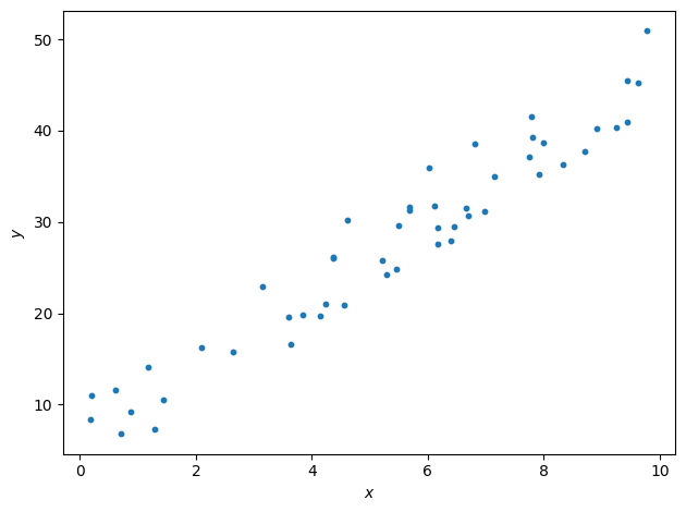
Now I see what you are thinking: it’s very straightforward (pun intended), it is just about fitting a straight line to the data. Yes. But this over-simplified setup is the starting point of our machine learning journey as it contains the basic mathematical machinery. Things will complicate soon, don’t worry.

So, what is linear regression to start with?

Definition 1

Linear regression is a model assuming a linear relationship between input variables and real-valued output variables.

• Input variables are called independent variables, or explanatory variables.

• The output variable is considered a dependent variable.

Linear regression is used to predict a real-valued output variable (dependent variable) based on the values of the input variables (independent variables).

Features and targets

Let’s now introduce terms more specific to the machine learning jargon and define some notations we will use through the course.

Terminology and Notation

• The input variables are called features and are denoted with \(x\).

• The output variable is the target and is denoted with \(y\).

• In supervised learning the dataset is called a training set.

• The number of training examples is denoted with \(m\).

• The \(i^{th}\) example is \((x^{(i)} , y^{(i)})\).

So the pair \((x^{(1)} , y^{(1)})\) is the first training sample from the data set.
And \((x^{(m)} , y^{(m)})\) refers to the last data point.

Warning

Here we start counting from one. When you will write code, the convention is to start at index zero. So your last sample will be of index m - 1. Keep this in mind.

When we refer to the entire list of all features and targets, we will use \(\boldsymbol{x}\) and \(\boldsymbol{y}\) respectively. Those are vectors.

We defined the input and output. In the middle is our model. We feed it first with all the input features and their associated known targets. This first step of supervised learning is called the training and we will see the mathematics behind it now. What we need first is a function that best maps input to output.

Hypothesis function

Definition 2

The hypothesis function, denoted \(h\), is a mapping function used to predict an output \(y^\text{pred}\) from an input \(x\):

\[\begin{equation*} y^\text{pred} = h(x) \end{equation*}\]

The hypothesis function is also known as decision function. It’s the mathematical core of a machine learning model.

In our simple case of linear regression in one dimension, our function \(h\) will be of the form:

(1)\[ h_\theta(x) = \theta_0 + \theta_1 \; x\]

The subscript \(\theta\) means that the function depends on the values taken by \(\theta_0\) and \(\theta_1\).

But what is behind those new variables?

Model parameters

Definition 3

The mapping function’s internal variables are called the model parameters. In this course, we denote them using the vector \(\theta\):

\[\begin{equation*} \boldsymbol{\theta} = \begin{pmatrix} \theta_0 \\ \theta_1 \\ \\ ... \\ \\ \theta_n \\ \end{pmatrix} \end{equation*}\]

In our case with the linear regression with one input feature, we need two parameters:

(2)\[\begin{split}\boldsymbol{\theta} = \begin{pmatrix} \theta_0 \\ \theta_1 \\ \end{pmatrix}\end{split}\]

The parameter \(\theta_1\) controls the slope of the line. The parameter \(\theta_0\) is compulsory to shift our data vertically. It’s called the offset, or intercept or bias.

Rephrasing the problem

We want to find the values of \(\theta_0\) and \(\theta_1\) that fit the data well. We could pick one training example \((x^{(k)} , y^{(k)})\) and derive the coefficients from there. But will this be the ‘best’ straight line to draw? The mathematical phrasing for such a task is to think in terms of errors. How do we calculate the errors? That’s a first question to ask. From a given vector of \(\theta\), how small are the errors? This picture below helps to visualize. From a given parameterization, that is to say a given tuple (\(\theta_0\) , \(\theta_1\) ), the mapping function will output continuous values of a predicted \(y^\text{pred}\) for a continuous range of \(x\). That is the dashed line. The errors are the (vertical) intervals between the \(y\) from the prediction and each data points.

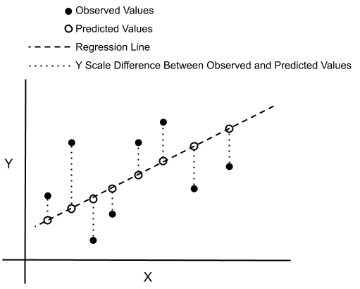
Fig. 1 : Visualization of errors (dotted vertical lines) between observed and predicted values.
Image: Don Cowan.

To see how well the prediction fit the data, we want the sum of all these errors to be as small as possible. In other words, we want to solve a minimization problem.

To avoid cancellation between positive and negative error values, we need to consider the errors as distance. Taking the absolute value or the square of those errors can do the trick: we get a positive number each time that will add up to the total error. Such evaluation is very similar to what is done for the minimum chi-square estimation. The name “chi” comes from the Greek letter \(\chi\), commonly used for the chi-square statistic. We will follow this protocol but in the ‘machine learning way.’ For this, we need to introducee a key concept: the cost function.