Learning Rate Schedulers
Contents
Learning Rate Schedulers#
Motivations#
We saw in previous lectures that the Gradient Descent algorithm updates the parameters, or weights, in the form:
The learning rate \(\alpha\) is kept constant through the whole process of Gradient Descent.
But we saw that the model’s performance could be drastrically affected by the learning rate value; if too small the descent would take ages to converge, too big it could explode and not converge at all. How to properly choose this crucial hyperparameter?
In the florishing epoch (pun intended) of deep learning, new optimization techniques have emerged. The two most influencial families are Learning Rate Schedulers and Adaptative Learning Rates.
Learning Rate Schedulers#
Definition 74
In a training procedure involving a learning rate, a learning rate scheduler is a method consisting of modifying the learning rate at the beginning of each iteration.
It uses a schedule function, which takes the current learning rate as input, along with a ‘time’ parameter linked with the increasing number of iterations, to output a new learning rate.
The updated learning rate is used in the optimizer.
Schedule refers to a timing; here it is the index number of the epoch, or iteration, that is incremented over time, i.e. the duration of the training.
Important
What is the difference between epoch, batches and iteration?
As we saw in Section Intuitive story-line of the gradient descent, an epoch is equivalent to the number of times the algorithm scans the entire data. It is a pass seeing the entire dataset. The batch size being the number of training samples, an iteration will be the number of batches needed to complete one epoch. Example: if we have 1000 training samples splits in batches of size 250 each, then it will take 4 iterations to complete one epoch.
Question
How should the learning rate vary? Should it increase? Decrease? Both?
Below are common learning schedules.
Power Scheduling#
The learning rate is modified according to:
where \(\alpha_0\) is the initial learning rate. The steps \(s\) and power \(c\) (usually 1) are hyperparameters. The learning rate drops at each step; e.g. after \(s\) steps it is divided by 2 (assuming \(c\) = 1).
Time-Based Decay Scheduling#
The time-based learning rate scheduler is often the standard (e.g. the default implementation in Keras library). It is controlled by a decay parameter \(d = \frac{\alpha_0}{N}\), where \(N\) is the number of epochs. It is similar (a particular case even) to the power scheduling:
As compared to a linear decrease, time-based decay causes learning rate to decrease faster upon training start, and much slower later (see graph below).
Exponential Decay Scheduling#
The exponential decay is defined as:
which will get the learning rate to decrease faster upon training start, and much slower later.
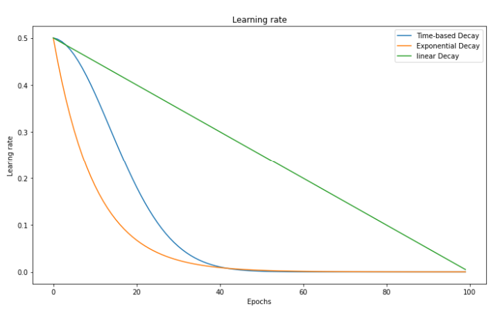
Fig. 51 . Evolution of the learning rate vs ‘time’ as the number of epochs for three schedulers: linear decrease, time-based decay and exponential decay.
Image: neptune.ai#
Step-based Decay Scheduling#
Also called piecewise constant scheduling, this approach first uses of a constant learning rate for a given number of epochs and then the learning rate is reduced:
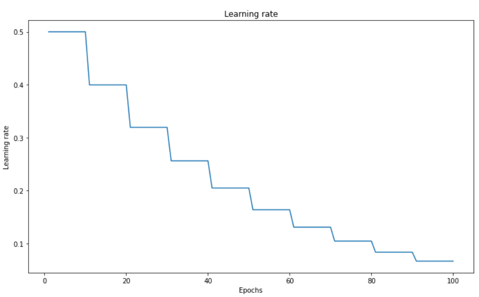
Fig. 52 . Step-based learning rate decay.
Image: neptune.ai#
Learn More
Guide to Pytorch Learning Rate Scheduling on Kaggle