Motivations

Let’s suppose we have a classification challenge looking like this:

Reminder: in linear and logistic regression, we took as hypothesis function a linear combination of the features with the \(\boldsymbol{\theta}\) parameters: \(h_\boldsymbol{\theta}(\boldsymbol{x}^{(i)}) = \sum_{j=0}^n \theta_j x^{(i)}_j = \boldsymbol{\theta} \cdot \boldsymbol{x}^{(i)}\)

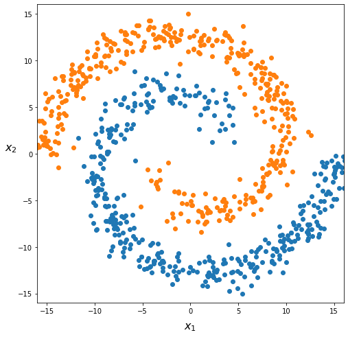
What can be a good hypothesis function? A linear hypothesis clearly cannot capture this pattern. So we will have to include higher degree polynomial terms in our hypothesis function. This would look like:

\[h_\boldsymbol{\theta}(\boldsymbol{x}) = \theta_0 + \theta_1 x_1 + \theta_2 x_2 + \theta_3 x_1 x_2 + \theta_4 x_1^2 x_2 + \theta_5 x_1^3 x_2 + \theta_6 x_1 x_2^2 + \cdots \]

If we include lots of polynomials, the hypothesis functions would eventually fit very complex data patterns. But there are issues.

First: how far should we go in polynomial degree? Moreover, we don’t know in advance which polynomial terms would be most useful for class separation. In the toy dataset above, with only two input features, we can visualize what’s happening in 2D. But in real applications with many features, we can’t simply “see” the decision boundary.

Second: with \(n\) input features \(x_1, x_2, \cdots, x_n\), adding quadratic terms will grow the amount of terms in \(h_\boldsymbol{\theta}(\boldsymbol{x})\) as \(\approx \frac{n^2}{2}\). With 10 input features, we will have more than 50 quadratic terms. With \(n=100\), we reach \(5000\) of terms! And we would not model complex patterns like the one above. Cubic combinations (\(x_1^3, x_1^2 x_2, x_1 x_2^2, \cdots \)) would add \(\mathcal{O}(n^3)\) new terms… This would become impracticable, likely overfit the data, and will definitely be too computationally expensive.

This is where artificial neural networks come in.

Exercise

1. Can you derive the number of quadratic and cubic terms mentioned above for a dataset with \(n\) input features?

2. How would you generalize this to a polynomial of degree \(d\)?