Bias & Variance: a Tradeoff

The bias and variance are the mathematical underpinnings of two distinct scenarios of mis-fit: underfitting and overfitting. Those situations are symptoms of high bias and high variance, respectively. Let’s first intuitively introduce under- and overfitting, then see how to diagnose them with convenient plots before presenting the bias-variance tradeoff. Last but not least, we will explore strategies to mitigate misfit and guide the model toward the optimal “sweet spot.”

Underfitting, overfitting

Let’s have a look at the three cases below:

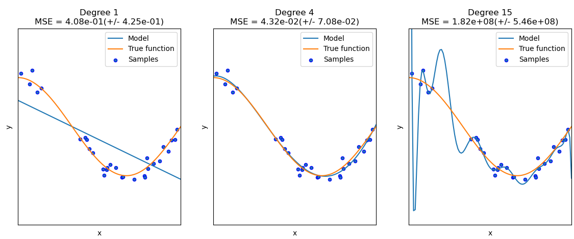
Fig. 22 : Example of several regression models attempting to fit data points (blue dots) generated from a true function (orange curve). A fitting attempt is depicted in blue for a polynomial of degree 1 (left), degree 4 (middle) and degree 15 (right).

_{Source: scikit-learn.org (with associated python code)}

What can we say qualitatively about the quality of those fits? The linear one on the left (polynomial of degree 1) is clearly missing out the main pattern of the data. No matter the slope and the offset, a straight line will never fit a wavy curve decently. This is a case of underfitting. The model is too simple. On the other hand, the fit on the right (polynomial of degree 15) is perfectly passing through all datapoints. Technically, the performance is excellent! But the model is abusing its numerous degrees of freedom and has done more than fitting the data: it captured all the fluctuations and the noise specific to the given dataset. If we regenerate samples from the orange true function, the blue curve with large oscillations will definitely not pass through the newly generated points. There will be substantial errors. The excess of freedom with the high-degree polynomial is a bit of a curse here. This is a case of overfitting: the model is over-specific to the given random variations in the dataset. In the middle model, we seem to find a good compromise with a polynomial function of degree 4.

Hope this gives you a feel of the underfitting and overfitting (or undertraining and overtraining, synonyms). Now let’s write the definitions!

Definition 35

Underfitting is a situation that occurs when a fitting procedure or machine learning algorithm is not capturing the general trend of the dataset.

Another way to put it: an underfit algorithm lacks complexity.

However, if we add too much complexity, we can fall in another trap: overfitting.

Definition 36

Overfitting is a situation that occurs when a fitting procedure or machine learning algorithm matches too precisely a particular collection of a dataset.

Overfitting is synonym of overtuned, overtweaked. In other words: the model learns the details and noise in the training dataset to the extent that it negatively impacts the performance of the model on a new dataset. This means that the noise or random fluctuations in the training dataset are picked up and learned as actual trends by the model. In machine learning, we look for general patterns and compromises: a good algorithm may not be perfectly classifying a given data set; it needs to accommodate and ignore rare outliers so that future predictions, on average, will be accurate.

The problem with overfitting is the future consequences once the machine learning algorithm receives additional data: it will very likely fail to generalize to new data.

Definition 37

In machine learning, generalization is the ability of a trained model to perform well on new, unseen data drawn from the same distribution as the training data.

Definition 38

The capacity of a model determines its ability to remember information about it’s training data.

Capacity is not a formal term, but it is linked to the number of degrees of freedom available to the model. A linear fit (two degrees of freedom) is limited to match a parabola. The model lacks capacity. However too much capacity can backfire! As in our example below, a model with many degrees of freedom will be so free that it is likely to fit some fluctuations. Problem.

But there is a trick! Let’s have those degrees of freedom (you get that with low-degree polynomials, we are stuck) but let’s add a constraint so as to tame the overfitting. This is called regularization.

Regularization to cope with overtraining

In Fig. 22, the model on the right that overfits the data is extremely wiggly. To produce such sharp peaks, some of the polynomial’s coefficients (the model parameters) must take on very large values to “force” the curve through the points. What if we added the values of the model parameters (the \(\boldsymbol{\theta}\) components) to the cost function? Since the cost is to be minimized, this could discourage the curve from becoming too wiggly. This is the idea behind the most common regularization techniques.

Definition 39

Regularization in machine learning is a processus consisting of adding constraints on a model’s parameters.

The two main types of regularization techniques are the Ridge Regularization (also known as Tikhonov regularization, albeit the latter is more general) and the Lasso Regularization.

Ridge Regression

The Ridge regression is a linear regression with an additional regularization term added to the cost function:

(39)\[ J(\theta) = \frac{1}{2m} \left[ \sum_{i=1}^{m} \left( h_\theta(x^{(i)}) - y^{(i)}\right)^2 + {\color{Maroon}\lambda \sum_{j=1}^n \theta_j^2} \right]\]

The hyperparameter \(\lambda\) controls the degree of regularization. If \(\lambda = 0\), the regularization term vanishes and we have a non-regularized linear regression. You can see the penalty imposed by the term \(\lambda\) will force the parameters \(\theta\) to be as small as possible; this helps avoiding overfitting. If \(\lambda\) gets very large, the parameters can be so shrinked that the model becomes over-simplified to a straight line and thus underfit the data.

Note

The factor \(\frac{1}{2}\) is used in some derivations of the regularization. This makes it easier to calculate the gradient, however it is only a constant value that can be compensated by the choice of the hyperparameter \(\lambda\).

Warning

The offset parameter \(\theta_0\) is not entering in the regularization sum.

In the litterature, the parameters are denoted with \(b\) for the offset (bias) and a vector of weight \(\vec{w}\) for the other parameters \(\theta_1, \theta_2, \cdots \theta_n\). Thus the regularization term is written:

(40)\[\lambda \left(\left\| \vec{w} \right\|_2\right)^2\]

The \(\ell_2\) norm is the Euclidian norm \(\left\| x \right\|_2 = \sqrt{x_0^2 + x_1^2 + \cdots + x_n^2}\).

with \(\left\| \vec{w} \right\|_2\) the \(\ell_2\) norm of the weight vector.

For logistic regression, the regularized cost function becomes:

(41)\[ C(\theta) = - \frac{1}{m} \sum^m_{i=1} \left[ \;\; y^{(i)} \log( h_\theta(x^{(i)} )) \;+\; (1- y^{(i)}) \log( 1 - h_\theta(x^{(i)} )) \;\;\right] + {\color{Maroon}\frac{\lambda}{2m} \sum_{j=1}^n \theta_j^2}\]

Lasso Regularization

The \(\ell_1\) norm is the sum of the magnitudes of the vectors. It is also called Manhattan or Taxicab norm.

Lasso stands for least absolute shrinkage and selection operator. Behind the long acronym is a regularization of the linear regression using the \(\ell_1\) norm. We denote Cost(\(\theta\)) the cost function, i.e. either the Mean Squared Error for linear regression or the cross-entropy loss function (19) for logistic regression. The lasso regression cost function is

(42)\[C(\theta) = \text{Cost(}{\theta}\text{)} + {\color{Maroon}\frac{\lambda}{2m} \sum_{j=1}^n | \theta_j | }\]

The regularizing term uses the \(\ell_1\) norm of the weight vector: \(\left\| \vec{w} \right\|_1\).

Warning

As regularization influences the parameters, it is important to first perform feature scaling before applying the regularization.

Which regularization method to use?

Each one has its pros and cons. As \(\ell_1\) (lasso) is a sum of absolute values, it is not differentiable and thus more computationally expensive. Yet \(\ell_1\) better deals with outliers (extreme values in the data) by not squaring their values. It is said to be more robust, i.e. more resilient to outliers in a dataset.

The \(\ell_1\) regularization, by shriking some parameters to zero (making them vanish and no more influencial), has feature selection built in by design. If this can be advantageous in some cases, it can mishandle highly correlated features by arbitrarily selecting one over the others.

Additional reading are provided below to deepen your understanding in the different regularization methods. Take home message: both methods combat overfitting.

Learn more

• A comparison of the pros and cons of Ridge (\(\ell_2\) norm) and lasso (\(\ell_1\) norm) regularization: “L1 Norms versus L2 Norms”, Kaggle

• Fighting overfitting with \(\ell_1\) or \(\ell_2\) regularization, neptune.ai

Bias & Variance: definitions

Underfitting and overfitting are symptoms of a fundamental modeling issue. This tension is captured by the notions of bias and variance. We will define them, see how they combine in the total error, and why it is not possible to reduce both simultaneously. This is the infamous dilemma of the bias–variance tradeoff.

Bias

The bias systematic error coming from wrong assumptions on the model.

Slight change of notations

Earlier in this course, we used \(h_\theta(x)\) as our model’s hypothesis function. For coherence in the notation, we will use \(\hat{f}_{\mathcal{D}}(x)\), which refers to the trained/fitted model, i.e., \(h_\theta(x)\) after training, with parameters \(\boldsymbol{\hat{\theta}}\) learned from the data \(\mathcal{D}\). So \(\hat{f}_{\mathcal{D}}\) is basically the post-training version of \(h_\theta\).

Definition 40

The bias measures how much, on average across different training sets \(\mathcal{D} = \mathcal{D}_1, \cdots, \mathcal{D}_N\), the model’s predictions \(\hat{f}_{\mathcal{D}_k}(x)\) deviate from the true underlying function \(f(x)\):

(43)\[\text{Bias}(x) = \mathbb{E}[\hat{f}_{\mathcal{D}}(x)] - f(x)\]

A highly biased model will most likely underfit the data.

Important

The true distribution \(P(X,Y)\) from which the data are drawn is unknown, so the true function \(f(x)\) cannot be observed directly. We can write it down, but we will never have direct access to it.

Variance

Definition 41

The variance is a measure of how sensitive the model’s predictions are to random fluctuations in the training data.

(44)\[\text{Variance}(x) = \mathbb{E}\Big[(\hat{f}_{\mathcal{D}}(x) - \mathbb{E}[\hat{f}_{\mathcal{D}}(x)])^2\Big]\]

As its name suggest, a model incorporating fluctuations in its design will change, aka vary, as soon as it is presented with new data (fluctuating differently). Variance is about the instability of the model due to training data variability.

A model with high variance is likely to overfit the data.

Using a larger training dataset will reduce the variance. However, extremely high-variance models may still fluctuate, but in general, more data helps.

Illustratively

Below is a good visualization of the two tendencies for both regression and classification:

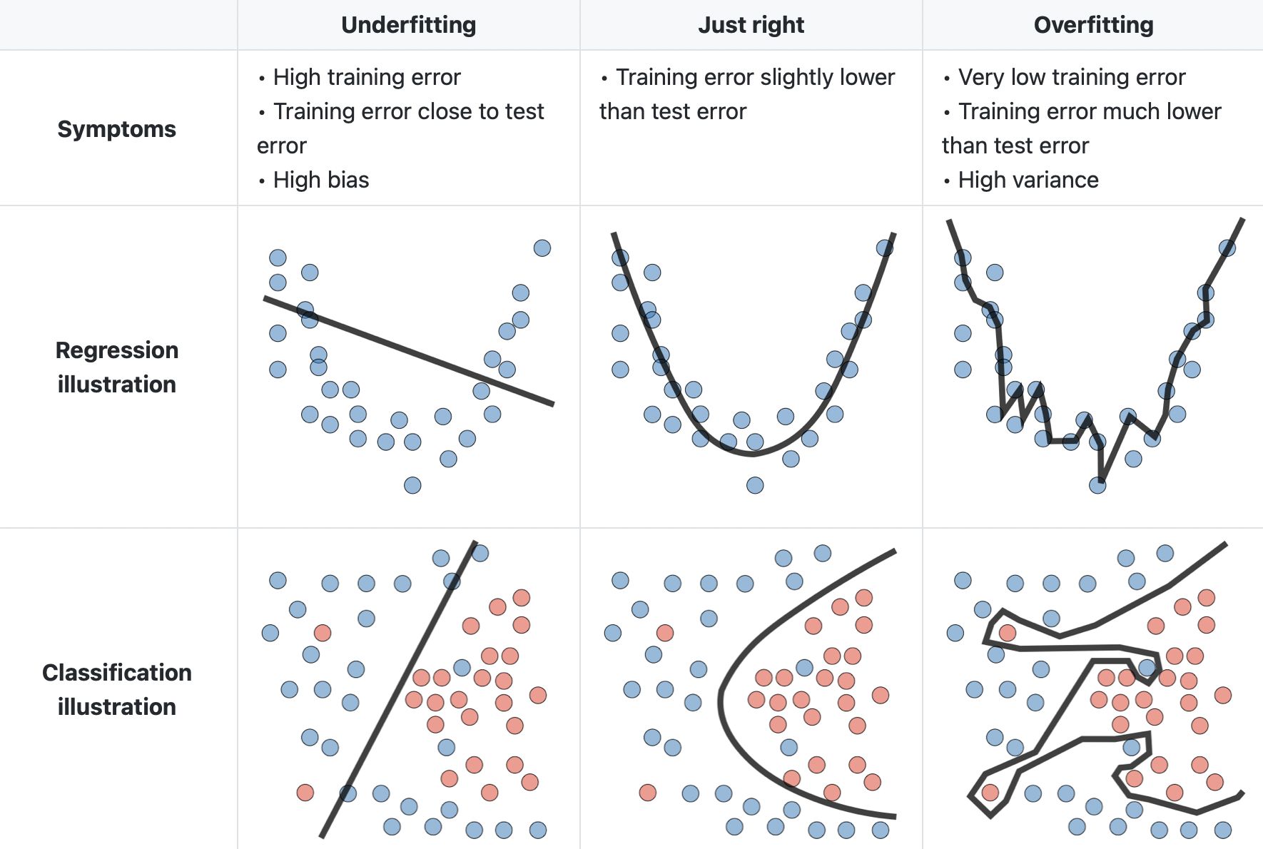
Fig. 23 : Illustration of situations of high bias (left) and high variance (right) for regression and classification.
_{Image: LinkedIn Machine Learning India}

We can see that the left column deals with models too simple, very low in capacity, so completely failing to get the main data patterns. As a result, we will have a high cost (or error) with data used during the training as well as new data points to test the generalization. No matter how many new data points we add. This is a high bias situation – model too simple – and it can be spotted with the fact that errors will be large on both the training and the testing datasets.

Now, if the capacity is increased – with a higher degree polynomial or advanced model architecture – we can get a high variance situation. In that case, the error on the training dataset will be small. For a moment, we can think the model is great! However, if we test the model with new, unseen-during-training data, the fluctuations will differ and thus we will get a large testing error. This is a high variance situation. In that case, the errors will be low on the training dataset but large on the testing dataset.

To see which situation we are in, we compare errors on the training and test sets.

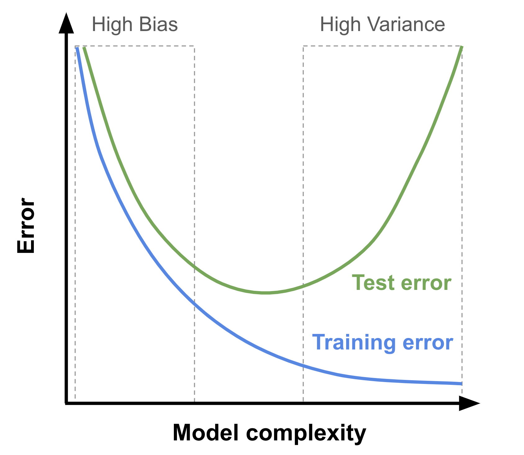
Fig. 24 Visualization of the error (cost function) with respect to the model’s complexity for the training and test sets. The ideal complexity is in the middle region where both the training and test errors are low and close to one another.
_{Image: from the author, inspired by David Ziganto}

Two takeaways from this:

1. The reduction of bias is done at the expend of an increase in variance. That’s unavoidable and we will soon see this both mathematically and practically

2. There is a golden mean, a zone where the model is compromising both on the bias and variance. That corresponds to the bottom of the test error. In this zone, the model captures the main pattern of the data and the generalization to new data is minimized.

Generalization error

Definition 42

The generalization error of a model quantifies its expected loss on new data drawn from the same distribution as the training set.

In other words, the generalization error reflects how well the model captures essential patterns in the training data and transfers them to give accurate predictions on unseen data.

Decomposition

The generalization error can be expressed as a sum of three errors:

(45)\[\text{Expected Test Error} = \underbrace{\text{Bias}^2}_{\text{systematic error}} + \underbrace{\text{Variance}}_{\text{sensitivity to data}} + \underbrace{\sigma^2}_{\text{irreducible noise}}\]

This is the (infamous) bias-variance decomposition.

As the equation shows, the generalization error is an “expectation” of the loss on the test dataset. Put differently, it is a theoretical average over all possible unseen samples. The first two terms in the sum are reducible with a smart choice of model complexity, as we saw before. The third term comes from the fact that data is noisy. Beyond careful data cleaning and smart preprocessing, there is little we can do: there will always be some noise. It’s irreducible.

Some of you may wonder (or have forgotten): why is the bias squared?

The best way to know is to derive yourself the bias-variance decomposition. But before, let’s note an important point on what is being averaged over here.

Two different kinds of “averages”

An important point to note here in the bias–variance decomposition: the expectation is not over examples in the dataset! It’s over different possible training datasets. Bias and variance are defined pointwise.

Let’s take one point \(x^\text{test}\) from our test data.

To get the bias and variance on that point \(x^\text{test}\), we need to:

• Train our model on dataset \(\mathcal{D}_1\) \(\rightarrow\) we get predictor \(\hat{f}_{\mathcal{D}_1}(x^\text{test})\)

• Train our model on dataset \(\mathcal{D}_2\) \(\rightarrow\) we get predictor \(\hat{f}_{\mathcal{D}_2}(x^\text{test})\)

• …

• Train our model on dataset \(\mathcal{D}_N\) \(\rightarrow\) we get predictor \(\hat{f}_{\mathcal{D}_N}(x^\text{test})\)

Now, we can define the following:

Definition 43

The expectation of a model at a point \(x\) is the average of the predictions \(\hat{f}_\mathcal{D}(x)\) over many training datasets \(\mathcal{D} = \mathcal{D}_1, \cdots, \mathcal{D}_N\).

(46)\[\mathbb{E}_\mathcal{D} [ \hat{f}_\mathcal{D}(x) ]\]

Mathematical derivation

There won’t be the answer here, but guidance is available on demand. Try it yourself first! (Guaranteed joy after solving it with your own brain.)

Hint on the noise

The true function \(f(x)\) defines the relationship between \(X\) and the targets \(y\). But there will be some deviation due to noise. We can model this with an error term \(\epsilon\):

(47)\[y = f(x) + \epsilon\]

We assumed it is normally distributed and with a standard deviation of \(\sigma\).

Hint on how to start

Start by writing the expression of an expectation of the error:

(48)\[\text{Expected Test Error} = \mathbb{E} \Big[ y^\text{test} - \hat{f}_\mathcal{D}(x^\text{test})\Big]\]

For the derivation, you can omit the ‘test’ upperscript to lighten the equations a bit.

Now? Expand this expression and use the properties you know about expectations and variances…

Hint on a useful relation

Recall that the variance of a random variable \(X\) can be written in two ways:

(49)\[\mathrm{Var}(X) = \mathbb{E} \big[ (X - \mathbb{E}[X])^2 \big] = \mathbb{E}[X^2] - \mathbb{E}[X]^2\]

You will need this!

 
 
 
 
 
 

Check it! (after you tried hard)

Below are two derivations:

• The very accessible and easy-to-follow format by Allen Akinkunle: The Bias-Variance Decomposition Demystified. The illustrations with simulated data are excellent to really grasp the tradeoff. I suggest opening a notebook and giving it a try!

• The thorough Lecture 12: Bias-Variance Tradeoff by Kilian Weinberger, from the course Machine Learning for Intelligent Systems taught at Cornell University.

Brain teaser
Would the decomposition Bias\(^2\) + Variance still hold for a loss that is not the MSE? 🤔