Gradient Descent in 1D

This concept is key in machine learning. We will see the procedure with our example. Recall that our goal is to find values for the model parameters so as to minimize the errors.

Before diving into the gradient descent, let’s ask ourselves: is there a way to solve this analytically? In the case of linear regression: yes. It is called the Normal Equation.

Analytical Solution: Normal Equation

Definition 6

The Normal Equation gives the exact solution for the parameters that minimize the mean squared error in linear regression. For a dataset with input matrix \(X\) and output vector \(\boldsymbol{y}\):

(5)\[\begin{equation} \theta = (X^T X)^{-1} X^T \boldsymbol{y} \end{equation}\]

Here, \(X\) includes a column of ones for the intercept term. This formula computes the optimal parameters directly.

In our 1D case with a single input feature, the parameters can also be written explicitly as:

(6)\[\begin{equation} \theta_1 = \frac{\sum_i (x_i - \bar{x})(y_i - \bar{y})}{\sum_i (x_i - \bar{x})^2}, \quad \theta_0 = \bar{y} - \theta_1 \bar{x} \end{equation}\]

While the Normal Equation is elegant and exact, it becomes computationally expensive for very large datasets and/or when the number of features grows. The gradient descent offers an iterative, approximate method that can scale to the enormous datasets typical in machine learning.

Intuitive story-line of the gradient descent

Going down a valley blanketed by thick fog

This poetical description may feel enigmatic, but it will make sense once you read the following.

Definition 7

Gradient descent is an iterative optimization algorithm to find the minimum of a function.

The 3D plot from the previous section on visualizing the cost function is misleading, as we will see that once we add input features we cannot have any visual of how the data landscape looks like (we are stuck with 3D vision, rarely 4D and that’s it). In a way, we are blind. Think of yourself walking from a point of the bowl-shaped surface but in the dark. How to reach the ‘valley’ where the cost function is minimum?

The idea behind gradient descent is to walk step by step following the slope of the cost function locally. In mathematical words: the partial derivatives of the cost function will give us the best direction to go towards the minimum. We don’t need to compute the cost for all point of the parameter space – it would require summing over all data samples for each possible value of the model parameters. This is not feasible. Instead, we will start at random. We pick a point in the vaste parameter space. That means a set of \(\boldsymbol{\theta} = \theta_0, \theta_1\) (in our 1D case). Then we get, for each \(\boldsymbol{\theta}\) component, the slope via its partial derivative. The core of the gradient descent is the update rule: the model parameters are recomputed with a shift that goes, by construction, in the direction of the descending gradients. And we repeat, until we reach a certain number of iterations predefined or until the partial derivatives gets to zero. In our simple 1D case, we know the existence of a unique minimum, so the cancellation of both partial derivatives mean that we found the optimal set of \(\theta_0\) and \(\theta_1\) that minimize the cost!

Before going over the pseudo-code, let’s define important terms that we will encounter very soon:

Terminology

Definitions

Hyperparameter
A model argument set before starting the machine learning algorithm.
Hyperparameters control the learning process.

Learning rate \(\alpha\)
Hyperparameter in an optimization algorithm that determines the step size at each iteration while moving toward a minimum of a loss function.
The learning rate is always a strictly positive number.

Epoch
In machine learning, an epoch is the number of passes of the entire training dataset the machine learning algorithm has completed.
The number of epochs is a hyperparameter controlling the number of passes of the algorithm.

The version of Gradient Descent introduced here is called Batch Gradient Descent. Later, we will see variations where a subset of the dataset – or even a single sample – is used to compute the partial derivatives of the cost function. For now, we consider the full dataset – one entire batch – summed over while taking each partial derivative.

Pseudo-code of gradient descent in 1D

The steps of the gradient descent algorithm for a linear regression with two parameters (i.e. in 1D) are written below in the form of pseudo-code.

This definition will be generalized in the next section with more parameters, from \(\theta_0\) to \(\theta_n\).

Algorithm 1 (Gradient Descent for Univariate Linear Regression)

 
Inputs

• Training data set with input features \(\boldsymbol{x}\) associated with their targets \(\boldsymbol{y}\):

\[\begin{equation*} x = \begin{pmatrix} x^{(1)} \\ x^{(2)} \\ \vdots \\ \\ x^{(m)} \end{pmatrix} \hspace{10ex} y = \begin{pmatrix} y^{(1)} \\ y^{(2)} \\ \vdots \\ \\ y^{(m)} \end{pmatrix} \end{equation*}\]

Hyperparameters

• Learning rate \(\alpha\)

• Number of epochs \(N\)  

Outputs
The optimized values of the parameters: \(\theta_0\) and \(\theta_1\), minimizing \(C(\theta_0 , \theta_1)\).  

1. Initialization: Set random values for \(\theta_0\) and \(\theta_1\)

2. While the exit conditions are not met:

   1. Compute the partial derivatives of the cost function:

   (7)\[\begin{split} \begin{align*} & \frac{\partial }{\partial \theta_0} C(\theta_0 , \theta_1) \\ & \frac{\partial }{\partial \theta_1} C(\theta_0 , \theta_1) \end{align*}\end{split}\]

   1. Apply the update rule to get the new parameters:

   (8)\[\begin{split}\begin{align*} &\\ \theta'_0 &= \theta_0-\alpha \frac{\partial}{\partial \theta_0} C\left(\theta_0, \theta_1\right) \\ \\ \theta'_1 &= \theta_1-\alpha \frac{\partial}{\partial \theta_1} C\left(\theta_0, \theta_1\right) \end{align*}\end{split}\]

            Reassign the new \(\theta\) parameters to prepare for next iteration

   (9)\[\begin{split}\begin{align*} \theta_0 &= \theta'_0 \\ \\ \theta_1 &= \theta'_1 \\ \end{align*}\end{split}\]

Exit conditions

• After the maximum number of epochs \(N\) is reached

• If both partial derivatives of the cost function tend to zero

An important point: the parameters are updated simultaneously. In other words, we should not use an already updated \(\theta_0\) when updating \(\theta_1\). The equations above are kept simple, but we can write the update rule more precisely by introducing an iteration index \(t\). The updated parameters at iteration \(t+1\) are:

(10)\[\begin{split} \theta_{0, \, t+1} &= \theta_{0, \, t}-\alpha \frac{\partial}{\partial \theta_0} C\left(\theta_{0, \, t}, \theta_{1, \, t}\right) \\ \\ \theta_{1, \, t+1} &= \theta_{1, \, t}-\alpha \frac{\partial}{\partial \theta_1} C\left(\theta_{0, \, t}, \theta_{1, \, t}\right) \end{split}\]

Each model parameter are updated according to the ‘state’ at the previous iteration.

In linear regression, the partial derivatives can be simplified.

Exercise

Knowing the form of the hypothesis function \(h_\theta(x)\) for linear regression and the definition of the cost function, rewrite the Equation (8) with the explicit partial derivatives.

Answer

\[\begin{align*} \theta'_0 &= \theta_0-\alpha \frac{1}{m} \sum_{i = 1}^m \left(h_\theta(x^{(i)})-y^{(i)}\right) \\ \\ \theta'_1 &= \theta_1-\alpha \frac{1}{m} \sum_{i = 1}^m \left(h_\theta(x^{(i)})-y^{(i)}\right) x^{(i)} \end{align*}\]

Details on demand during office hours.

Important
Note that at the step 2.1., there is an implicit loop over all training data samples, as it is required by the cost function.

Why a minus sign before alpha?

This illustration helps see why the minus sign in Equation (8) is necessary.

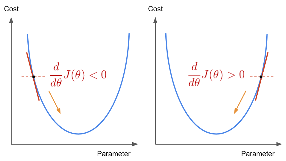
Fig. 3 : The sign of the cost function’s derivative changes for two different parameter values either lower (left) or greater (right) than the parameter value for which the cost function is minimized.
_{Image from the author}

If our parameter is randomly picked on the left side of the U-shaped parabola, the partial derivatives will be negative. As the learning rate is always positive, the incremental update \(-\alpha \frac{d}{d \theta} C(\theta)\) will thus be positive. We will add an increment to our parameter. At the next iteration, we will have a new parameter \(\theta\) closer to the one we look for. The reverse goes with the other side of the curve: with a positive derivative, we will decrease our parameter and slide to the left. All the time we go ‘downhill’ towards the minimum.

Graphical Visualization

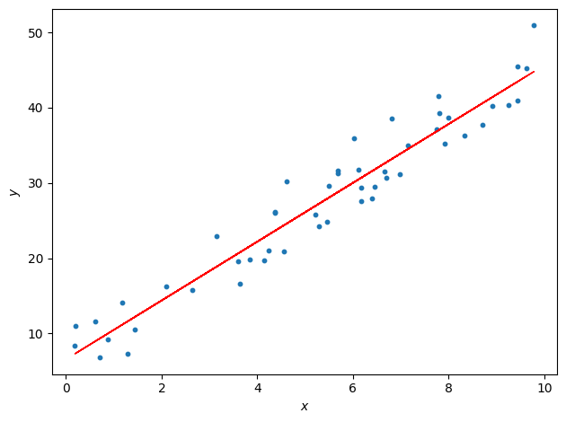
When computing the gradient descent for linear regression, we get new parameters so we can draw a candidate straight line to fit the data. With proper tuning (more on this later), we reach the ideal fit, minimizing the cost function.

Fig. 4 Animation of the gradient descent. At each generation a new set of parameters are computed. In this picture \(m\) corresponds to \(\theta_1\) and the constant \(c\) to \(\theta_0\). Sometimes they are also referred to the slope and intercept respectively.
_{Source GIF: Medium}

In our example, the best linear fit will be:

How to picture this in the \(\theta\) parameter space? For this, contour and 3D plot are handy. Below, the new parameters’trajectory (red points) are “descending” towards the minimum of the cost function:

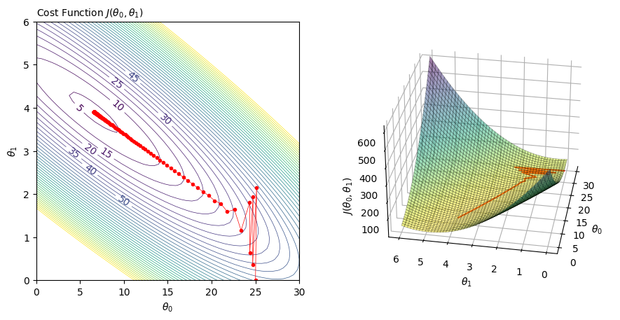
Fig. 5 Contour plot (left) and 3D rendering (right) of the cost function with respect to the values of the \(\theta\) parameter. The red dots are the intermediary values of the parameters at a given iteration of the gradient descent. You can see that it converges toward the minimum of the cost function.

We will discuss the presence of the zig-zag behaviour in the later section Learning Rate.

This was the gradient descent in one dimension. How can we generalize to \(n\) dimensions? This is what the next section will (un)cover.