Backpropagation Algorithm

Before Diving Into The Math

Ingredients

The forward propagation, or forward pass, will fill the network with values for all bias nodes and activation units. That includes the last layer of activation units, so the forward pass provides predictions.

We saw the loss function as the mathematical tool to compare the predictions with their associated observed values for a sample (and the cost function aggregates this for all data samples).

Then we are familiar with the gradient descent procedure, which gives at each iteration the positive or negative amount to correct the weights to eventually get a model that fits to the data.

For a neural network, there are lots of knobs to tweak! Luckily, an efficient technique called backpropagation is able to compute the gradient of the network’s error for every single model parameter.

Definition

Definition 63

Backpropagation, short for backward propagation of errors, is an algorithm working from the output nodes to the input nodes of a neural network using the chain rule to compute how much each activation unit contributed to the overall error.

It automatically computes error gradients to then repeatedly adjust all weights and biases to reduce the overall error.

Chain Rule Refresher

A little interlude and refresher of the chain rule will not hurt.

Definition 64

Let \(f\) and \(g\) be functions. For all \(𝑥\) in the domain of \(g\) for which \(g\) is differentiable at \(x\) and \(f\) is differentiable at \(g(x)\), the derivative of the composite function:

(80)\[\begin{equation} h(x) = f(g(x)) \end{equation}\]

is given by

(81)\[\begin{equation} h'(x) = \frac{\mathrm{d} \; f(g(x)) }{\mathrm{{\color{Maroon}d}} \; {\color{Maroon}g(x)}} \;\cdot \; \frac{\mathrm{{\color{Maroon}d}} \; {\color{Maroon}g(x)}}{\mathrm{d} \; x} = f'\left(g(x)\right) \;\cdot \; g'(x) \end{equation}\]

You can see above from the colouring that the inserted denominator and numerator of the composed function cancel out. All good. Now your turn with three functions (and that will be useful for the rest of the lecture).

Warning

The prime notation \(f'(\square)\) can be error-prone. It is the derivative with respect to \(\square\) as the variable, i.e. as a block on its own (even if it depends on other variables).

\[\begin{equation*} \frac{\mathrm{d} f(\square)}{\mathrm{d} \square} = f'(\square ) \end{equation*}\]

Exercise

What would be the chain rule for three functions?

(82)\[\begin{equation} k(x) = h(f(g(x))) \end{equation}\]

Check your answer

(83)\[\begin{split}\begin{align*} k'(x) &= \; \frac{\mathrm{d} \; h(f(g(x)))}{\mathrm{{\color{BurntOrange}d}} \; {\color{BurntOrange}f(g(x))}} &\;\cdot\;& \frac{\mathrm{{\color{Peach}d}} \; {\color{Peach}f(g(x))} }{\mathrm{{\color{Maroon}d}} \; {\color{Maroon}g(x)}} &\;\cdot \;& \frac{\mathrm{{\color{Maroon}d}} \; {\color{Maroon}g(x)}}{\mathrm{d} \; x} \\[1ex] &= \; h'(f(g(x))) &\;\cdot\;& f'\left(g(x)\right) &\;\cdot \;& g'(x)\\ \end{align*}\end{split}\]

Three functions: three derivative terms.
We work from the outside first, taking one derivative at a time.

Main Steps

Before diving into a more mathematical writing, let’s just list the main steps of backpropagation. We will detail steps 2 and 3 very soon:

Algorithm 5 (Backpropagation)

Inputs
Training data set \(X\) of \(m\) samples with each \(n\) input features, associated with their targets \(y\)

Hyperparameters

• Learning rate \(\alpha\)

• Number of epochs \(N\)

Start

Step 0: Weight initialization

Step 1: Forward propagation:
\(\qquad \qquad \qquad \qquad \Rightarrow\) get list of \(m\) predictions \(\boldsymbol{\hat{y}}\)

Step 2: Backpropagation:
\(\qquad \qquad \qquad \qquad \Rightarrow\) get all errors \(\boldsymbol{\delta}^{(\ell)}_{n^{\ell}}\\[2ex]\)
\(\qquad \qquad \qquad \qquad \Rightarrow\) sum errors and get all cost derivatives:

\[\frac{\partial \text{ Cost}}{\partial W^{(\ell)}} \qquad ; \qquad \frac{\partial \text{ Cost}}{\partial \boldsymbol{b}^{(\ell)}}\]

Step 3: Gradient Descent steps to update weights & biases:

\[\begin{split}\begin{align*} W^{(\ell)} &\leftarrow W^{(\ell)} - \alpha \frac{\partial \text{ Cost}}{\partial W^{(\ell)}} \\[1ex] \boldsymbol{b}^{(\ell)} &\leftarrow \boldsymbol{b}^{(\ell)} - \alpha \frac{\partial \text{ Cost}}{\partial \boldsymbol{b}^{(\ell)}} \end{align*} \end{split}\]

End of epoch, repeat step 1 - 3 until/unless:

Exit conditions:

• Number of epochs \(N^\text{epoch}\) is reached

• If all derivatives are zero or below a small threshold

Computations

Now there will be math.

What is the goal?

Always a good question to start. We want to tweak the weights \(\boldsymbol{W}\) and biases \(\boldsymbol{b}\) so that the network predictions \(\boldsymbol{\hat{y}}\) get as close as they can be to the observed values \(\boldsymbol{y}\). In other words, we want to know how to change the weights and biases so that we minimize the cost:

(84)\[ \min_{\boldsymbol{W},\boldsymbol{b}} \text{ Cost}(\boldsymbol{W},\boldsymbol{b})\]

For this, we will need the partial derivatives of the cost function with respect to the parameters we want to optimize.

With derivatives, especially partial ones, it’s crucial to ask the question:

What varies here and with respect to what?
How will the numerator entity change as the denominator change?
Here we want to know how to vary the weights and biases so that the cost gets lower:

(85)\[\begin{gathered} \frac{\partial \text{ Cost}( \boldsymbol{W},\boldsymbol{b} )}{\partial \boldsymbol{W}} \qquad \frac{\partial \text{ Cost}( \boldsymbol{W},\boldsymbol{b} )}{\partial \boldsymbol{b}} \end{gathered}\]

Warning

Most mathematical textbooks have \(x\) as the varying entity while explaining the derivative business. It can be here misleading with our notation as we use \(\boldsymbol{x}\) as well. But in our case, \(\boldsymbol{x}\) are the input features. They are given. They will not change (unless you bring new data, but there will still be given numbers you’re not supposed to tweak). What we want is to vary the weights \(\boldsymbol{W}\) and biases \(\boldsymbol{b}\) to find optimized values for which the error is minimum, i.e. the model predicts a \(\hat{y}\) as close as possible as the real target \(y\).

Equation (85) can be overwhelming, especially given the numerous quantities of weights and biases in a neural network. No panic! Thanks to backpropagation, there will be a way to not only get those derivatives, but also be very efficient in their computation.

Notations

Let’s first rewrite the activation unit equation as a function of a function. We saw in the previous lecture:

(86)\[\boldsymbol{a}^{(\ell)} = f\left( \; \boldsymbol{a}^{(\ell -1)} \;W^{(\ell)} \;+\; \boldsymbol{b}^{(\ell)} \;\right) \;,\]

with \(f\) the node’s activation function and \(\ell\) is the current layer of the activation unit. Let’s split the notation by defining a function, noted \(z\), for the sum only:

(87)\[\boldsymbol{z}^{(\ell)} = \boldsymbol{a}^{(\ell-1)} W^{(\ell)} + \boldsymbol{b}^{(\ell)}\]

This would be called the “weighted sum plus bias.” So then each activation unit can be computed as:

(88)\[\boldsymbol{a}^{(\ell)} = f(\boldsymbol{z}^{(\ell)})\]

We will denote the loss function through a general form as \(L\):

(89)\[L\left(\hat{y}^{(i)}, y^{(i)}\right) \]

It is computed for each sample instance \(\left\{ \boldsymbol{x^{(i)}}, y^{(i)} \right\}\), with \(\boldsymbol{x^{(i)}} = (x_1^{(i)}, x_2^{(i)}, \cdots, x_n^{(i)})\) being one row of input features and \(y^{(i)}\) the associated target.

The cost is the sum of the losses over all data instances \(m\). To make the equations of the following section more readable, the sum will be written without instance indices as superscript (already used for the layer number); it is implied that it is the sum over all data instances.

(90)\[\text{Cost} = \frac{1}{m} \sum_{i=1}^m L\left(\hat{y}^{(i)}, y^{(i)}\right) = \frac{1}{m} \sum L\left(\boldsymbol{\hat{y}}, \boldsymbol{y}\right)\]

Here \(\boldsymbol{\hat{y}}\) and \(\boldsymbol{y}\) are in bold to show there are lists (of \(m\) elements).

How can we express the final output \(\boldsymbol{\hat{y}}\)?
Let’s take a similar network as the one in the previous lecture but layers are labeled from the last one (right) in decreasing order:

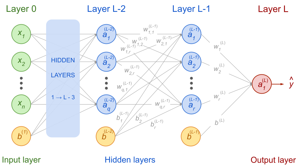
Fig. 54 . Feedforward neural network with the notations for the
last, before last and before before last layers.
_{Image from the author}

The final prediction \(\hat{y}^{(i)}\) is the output of the activation unit in the last layer:

(91)\[\hat{y}_1^{(i)} = a_1^{(L,i)} \]

In the network above, there is only one activation unit, so we can omit the subscript. But there is a prediction for each data sample. The collection of \(m\) predictions will be a column vector \(\boldsymbol{\hat{y}}\). So let’s write the predictions and activation units in bold:

(92)\[\boldsymbol{\hat{y}} = \boldsymbol{a}^{(L)}\]

So far, so good. Now the cost.

---

The cost function is obtained using Equations (88), (90) and (92):

(93)\[\text{Cost} = \frac{1}{m} \sum L\left(\boldsymbol{\hat{y}}, \boldsymbol{y}\right) = \frac{1}{m} \sum L\left(\boldsymbol{a}^{(L)}, \boldsymbol{y}\right) = \frac{1}{m} \sum L(f(\boldsymbol{z}^{(L)}), \boldsymbol{y}) \]

---

Let’s joyfully take the derivatives of that sandwich of functions! Now do you get the chain rule refresher?

We will use it, starting with the last layer and see how things simplify (yes, it will). Then we will backpropagate layer after layer.

The backward walk

As its name indicates, the backward propagation proceeds from the last to the first input layer. Let’s write the derivative of the cost function with respect to the weight matrix of the last layer:

(94)\[\frac{\partial \text { Cost }}{\partial \; W^{(L)}} = \; \frac{1}{m} \sum \; \frac{\partial L(f(\boldsymbol{z}^{(L)}), \boldsymbol{y})}{\partial \; W^{(L)}} = \; \frac{1}{m} \sum \; \frac{\partial L(f(\boldsymbol{z}^{(L)}), \boldsymbol{y})}{\partial f(\boldsymbol{z}^{(L)})} \; \cdot \; \frac{\partial f(\boldsymbol{z}^{(L)})}{\partial \boldsymbol{z}^{(L)}} \; \cdot \; \frac{\partial \boldsymbol{z}^{(L)}}{\partial W^{(L)}} \]

We can simplify things. The first term is the derivative of the loss function with \(f(\boldsymbol{z}^{(L)}) = \boldsymbol{a}^{(L)}\) as argument. It’s a value here, computed with all weights values. Same for the second term: it is the derivative of the activation function taken for the value \(\boldsymbol{z}^{(L)}\). For the third, we use the definition in Equation (87) that yields: \(\left( \boldsymbol{z}^{(L)} \right)^{\prime} = \boldsymbol{a}^{(L-1)}\). We can write:

(95)\[\frac{\partial \text { Cost }}{\partial W^{(L)}} = \; \frac{1}{m}\; \sum \;\; L^{\prime}(\boldsymbol{a}^{(L)}, \boldsymbol{y}) \;\cdot \; f^{\prime}(\boldsymbol{z}^{(L)}) \;\cdot \; \boldsymbol{a}^{(L-1)}\]

This is known! We can compute a value for this derivative!

Now let’s proceed to the before last layer. Using the chain rule as usual:

(96)\[\begin{split}\begin{align*} & \frac{\partial \text { Cost }}{\partial W^{(L-1)}} = \; \frac{1}{m} \\[1ex] & \sum \; \frac{\partial L(f(\boldsymbol{z}^{(L)}), \boldsymbol{y})}{\partial f(\boldsymbol{z}^{(L)})} \; \cdot \; \frac{\partial f(\boldsymbol{z}^{(L)})}{\partial \boldsymbol{z}^{(L)}} \; \cdot \; \frac{\partial \boldsymbol{z}^{(L)}}{\partial \boldsymbol{a}^{(L-1)}} \; \cdot \; \frac{\partial \; \boldsymbol{a}^{(L-1)} }{\partial\;\boldsymbol{z}^{(L-1)} } \; \cdot \; \frac{\partial \; \boldsymbol{z}^{(L-1)} }{\partial\;W^{(L-1)} } \end{align*}\end{split}\]

The two first terms are identical as in Equation (94). Using the definitions of \(\boldsymbol{a}\) and \(\boldsymbol{z}\) we have:

(97)\[\begin{gathered} \frac{\partial \boldsymbol{z}^{(L)}}{\partial \boldsymbol{a}^{(L-1)}} \;=\; W^{(L)} \qquad,\qquad \frac{\partial \; \boldsymbol{a}^{(L-1)} }{\partial\;\boldsymbol{z}^{(L-1)} } \;=\; f'(\boldsymbol{z}^{(L-1)}) \qquad,\qquad \frac{\partial \; \boldsymbol{z}^{(L-1)} }{\partial\;W^{(L-1)} } \;=\; \boldsymbol{a}^{(L-2)} \end{gathered}\]

Therefore:

(98)\[\frac{\partial \text { Cost }}{\partial W^{(L-1)}} = \; \frac{1}{m} \; \sum \;\; L^{\prime}(\boldsymbol{a}^{(L)}, \boldsymbol{y}) \;\cdot \; f^{\prime}(\boldsymbol{z}^{(L)}) \;\cdot \; W^{(L)} \;\cdot \; f'(\boldsymbol{z}^{(L-1)}) \;\cdot \; \boldsymbol{a}^{(L-2)}\]

You can check yourself that for the derivative with respect to \(W^{(L-2)}\) we will have:

(99)\[\begin{split}\begin{align*} & \frac{\partial \text { Cost }}{\partial W^{(L-2)}} = \; \frac{1}{m} \\[1ex] & \sum \;\; L^{\prime}(\boldsymbol{a}^{(L)}, \boldsymbol{y}) \;\cdot \; f^{\prime}(\boldsymbol{z}^{(L)}) \;\cdot \; W^{(L)} \;\cdot \; f'(\boldsymbol{z}^{(L-1)}) \;\cdot \; W^{(L-1)} \;\cdot \; f'(\boldsymbol{z}^{(L-2)}) \;\cdot \; \boldsymbol{a}^{(L-3)} \end{align*}\end{split}\]

We can see a pattern here!

We go all the way to the first hidden layer 1 (scroll to the right):

(100)\[\frac{\partial \text { Cost }}{\partial W^{(1)}} = \; \frac{1}{m} \; \sum \;\; L^{\prime}(\boldsymbol{a}^{(L)}, \boldsymbol{y}) \;\cdot \; f^{\prime}(\boldsymbol{z}^{(L)}) \;\cdot \; W^{(L)} \;\cdot \; f'(\boldsymbol{z}^{(L-1)}) \;\cdot \; W^{(L-1)} \;\cdot \; f'(\boldsymbol{z}^{(L-2)}) \;\cdot \; W^{(L-2)} \;\cdots\; W^{(2)} \;\cdot \; f'(\boldsymbol{z}^{(1)}) \;\cdot \; \boldsymbol{x}\]

where \(\boldsymbol{x} = \boldsymbol{a}^{(0)}\) as defined in the previous lecture in Equation (63).

Recursive error equation

We can write Equations (95), (98) and (99) by introducing an error term \(\boldsymbol{\delta}\). For the last layer it is defined as the product of the first two partial derivatives times the activation unit’s value at the previous layer. For the following (previous) layers it would be:

(101)\[\begin{split}\begin{align*} \boldsymbol{\delta}^{(L)} &=\; L^{\prime}(\boldsymbol{a}^{(L)}, \boldsymbol{y}) \cdot f^{\prime}(\boldsymbol{z}^{(L)}) & \rightarrow \frac{\partial \text{ Cost}}{\partial W^{(L)}} &= \; \frac{1}{m} \; \sum \;\boldsymbol{\delta}^{(L)} \;\cdot\; \boldsymbol{a}^{(L-1)}\\[2ex] \boldsymbol{\delta}^{(L-1)} &=\; \boldsymbol{\delta}^{(L)} \cdot\; W^{(L)} \cdot\; f'(\boldsymbol{z}^{(L-1)}) & \rightarrow \frac{\partial \text{ Cost}}{\partial W^{(L-1)}} &= \; \frac{1}{m} \; \sum \;\boldsymbol{\delta}^{(L-1)} \;\cdot\; \boldsymbol{a}^{(L-2)}\\[2ex] \boldsymbol{\delta}^{(L-2)} &=\; \boldsymbol{\delta}^{(L-1)} \cdot\; W^{(L-1)} \;\cdot\; f'(\boldsymbol{z}^{(L-2)}) & \rightarrow \frac{\partial \text{ Cost}}{\partial W^{(L-2)}} &= \; \frac{1}{m} \; \sum \;\boldsymbol{\delta}^{(L-2)} \;\cdot\; \boldsymbol{a}^{(L-3)}\\ \end{align*} \end{split}\]

This is recursive because errors from the current layer are used to evaluate error signals in a previous layer. We can write the recursive formula for any partial derivative in layer \(\ell\) as:

(102)\[\frac{\partial \text{ Cost}}{\partial W^{(\ell)}} = \;\;\; \frac{1}{m} \; \sum \quad\boldsymbol{\delta}^{(\ell)} \;\cdot\; \boldsymbol{a}^{(\ell-1)}\]

What about the biases?
This is left as exercise for training.

Exercise

Express the partial derivatives of the cost with respect to the biases \(\boldsymbol{b}^{(\ell)}\).

Hint: start with the last layer \(L\) as done previously with the weights.

Check your answer

The formula is essentially the same as for the weights, at the difference that the partial derivative of \(\boldsymbol{z}^{(\ell)}\) with respect to \(\boldsymbol{b}^{(\ell)}\) is 1:

\[\begin{equation*} \frac{\partial \boldsymbol{z}^{(\ell)}}{\partial \boldsymbol{b}^{(\ell)}} = 1 \end{equation*}\]

Thus:

(103)\[\begin{split}\begin{align*} \boldsymbol{\delta}^{(L)} &=\; L^{\prime}(\boldsymbol{a}^{(L)}, \boldsymbol{y}) \cdot f^{\prime}(\boldsymbol{z}^{(L)}) & \longrightarrow & \quad \frac{\partial \text {Cost}}{\partial \boldsymbol{b}^{(L)}} &=& \; \frac{1}{m} \quad \sum \quad\boldsymbol{\delta}^{(L)} \\[1ex] \boldsymbol{\delta}^{(L-1)} &= \; \boldsymbol{\delta}^{(L)} \cdot\; W^{(L)} \cdot\; f'(\boldsymbol{z}^{(L-1)}) & \longrightarrow & \quad \frac{\partial \text {Cost}}{\partial \boldsymbol{b}^{(L-1)}} &=& \; \frac{1}{m} \quad \sum \quad\boldsymbol{\delta}^{(L-1)} \\[1ex] \boldsymbol{\delta}^{(L-2)} &= \; \boldsymbol{\delta}^{(L-1)} \cdot\; W^{(L-1)} \;\cdot\; f'(\boldsymbol{z}^{(L-2)}) & \longrightarrow & \quad \frac{\partial \text {Cost}}{\partial \boldsymbol{b}^{(L-2)}} &=& \; \frac{1}{m} \quad \sum \quad\boldsymbol{\delta}^{(L-2)} \\[1ex] & \quad\cdots & & \cdots & \\[1ex] \boldsymbol{\delta}^{(1)} &= \; \boldsymbol{\delta}^{(2)} \cdot\; W^{(2)} \;\cdot\; f'(\boldsymbol{z}^{(1)}) & \longrightarrow & \quad \frac{\partial \text {Cost}}{\partial \boldsymbol{b}^{(1)}} &=& \; \frac{1}{m} \quad \sum \quad\boldsymbol{\delta}^{(1)} \\[1ex] \end{align*} \end{split}\]

Weights and biases update

After backpropagating, each weight and bias in the network is adjusted in proportion to how much it contributes to overall error.

The equations are different as in the section Main Steps as we keep here the ‘lite’ notations introduced above. The indices referring to the row and column of each weight/bias are implied for smoother reading. But remember that \(W\) and \(b\) are matrices and vectors respectively.

(104)\[\begin{split}\begin{align*} W^{(\ell)} &\leftarrow W^{(\ell)} - \alpha \frac{\partial \text{ Cost}}{\partial W^{(\ell)}} \\[1ex] \boldsymbol{b}^{(\ell)} &\leftarrow \boldsymbol{b}^{(\ell)} - \alpha \frac{\partial \text{ Cost}}{\partial \boldsymbol{b}^{(\ell)}} \end{align*}\end{split}\]

Memoization (and it’s not a typo)

This is a computer science term. It refers to an optimization technique to make computations faster, in particular by reusing previous calculations. This translates into storing intermediary results so that they are called again if needed, not recomputed. Recursive functions by definition reuse the outcomes of the previous iteration at the current one, so memoization is at play.

Let’s illustrate this point by writing the derivative equations for a network with one output layer and three hidden layers:

(105)\[\begin{split}\begin{align*} \frac{\partial \text { Cost }}{\partial W^{(4)}} &= \; \frac{1}{m} \; \sum \; {\color{OliveGreen}L^{\prime}(\boldsymbol{a}^{(4)}, \boldsymbol{y}) \cdot f^{\prime}(\boldsymbol{z}^{(4)})} \cdot \boldsymbol{a}^{(3)} \\[2ex] \frac{\partial \text { Cost }}{\partial W^{(3)}} &= \; \frac{1}{m} \; \sum \; {\color{OliveGreen}L^{\prime}(\boldsymbol{a}^{(4)}, \boldsymbol{y}) \cdot f^{\prime}(\boldsymbol{z}^{(4)})} \cdot {\color{Cyan}W^{(4)} \cdot f'(\boldsymbol{z}^{(3)})} \cdot \boldsymbol{a}^{(2)} \\[2ex] \frac{\partial \text { Cost }}{\partial W^{(2)}} &= \; \frac{1}{m} \; \sum \; {\color{OliveGreen}L^{\prime}(\boldsymbol{a}^{(4)}, \boldsymbol{y}) \cdot f^{\prime}(\boldsymbol{z}^{(4)})} \cdot {\color{Cyan}W^{(4)} \cdot f'(\boldsymbol{z}^{(3)})} \cdot {\color{DarkOrange}W^{(3)} \cdot f'(\boldsymbol{z}^{(2)})} \cdot \boldsymbol{a}^{(1)} \\[2ex] \frac{\partial \text { Cost }}{\partial W^{(1)}} &= \; \frac{1}{m} \; \sum \; {\color{OliveGreen}L^{\prime}(\boldsymbol{a}^{(4)}, \boldsymbol{y}) \cdot f^{\prime}(\boldsymbol{z}^{(4)})} \cdot {\color{Cyan}W^{(4)} \cdot f'(\boldsymbol{z}^{(3)})} \cdot {\color{DarkOrange}W^{(3)} \cdot f'(\boldsymbol{z}^{(2)})} \cdot W^{(2)} \cdot f'(\boldsymbol{z}^{(1)}) \cdot \boldsymbol{x}\\[2ex] \end{align*}\end{split}\]

The reoccuring computations are highlighted in the same colour. Now you can get a sense of the genius behind neural network: although there are many computations, a lot of calculations are reused as we move backwards through the network. With proper memoization, the whole process can be very fast.

Summary on backpropagation

The backpropagation of error is a recursive algorithm reusing the computations from last until first layer to compute how much each activation unit and bias node contribute to the overall error. The idea behind backpropagation is to share the repeated computations wherever possible. Let’s write again the steps with the key equations:

Algorithm 6 (Backpropagation)

Inputs
Training data set \(X\) of \(m\) samples with each \(n\) input features, associated with their targets \(\boldsymbol{y}\)

Hyperparameters

• Learning rate \(\alpha\)

• Number of epochs \(N\)

Start

Step 0: Weight initialization

Step 1: Forward propagation
\(\qquad \quad \Rightarrow\) get list of \(m\) predictions \(\boldsymbol{\hat{y}}\)

(106)\[\begin{equation} f(\boldsymbol{z}^{(L)}) = \boldsymbol{a}^{(L)} = \boldsymbol{\hat{y}} \end{equation}\]

Step 2: Backpropagation
\(\qquad \quad \Rightarrow\) get the cost:

(107)\[\begin{equation} \text{Cost} = \; \frac{1}{m} \; \sum L(f(\boldsymbol{z}^{(L)}), \boldsymbol{y}) \end{equation}\]

\(\qquad \quad \Rightarrow\) get all errors:

(108)\[\begin{equation} \boldsymbol{\delta}^{(L)} =\; L^{\prime}(\boldsymbol{a}^{(L)}, \boldsymbol{y}) \cdot f^{\prime}(\boldsymbol{z}^{(L)}) \end{equation}\]

(109)\[\begin{equation} \qquad \;\; \boldsymbol{\delta}^{(\ell)} = \; \boldsymbol{\delta}^{(\ell+1)} \;\cdot\; W^{(\ell+1)} \;\cdot\; f'(\boldsymbol{z}^{(\ell)}) \end{equation}\]

\(\qquad \quad \Rightarrow\) sum errors and get all cost derivatives:

\[\begin{split}\begin{align*} \frac{\partial \text{ Cost}}{\partial W^{(\ell)}} &= \;\frac{1}{m} \; \sum \; \boldsymbol{\delta}^{(\ell)} \;\cdot\; \boldsymbol{a}^{(\ell-1)}\\[2ex] \frac{\partial \text {Cost}}{\partial \boldsymbol{b}^{(\ell)}} &= \; \frac{1}{m} \; \sum \quad\boldsymbol{\delta}^{(\ell)} \end{align*}\end{split}\]

Step 3: Gradient Descent
\(\qquad \quad \Rightarrow\) update weights & biases:

\[\begin{split}\begin{align*} W^{(\ell)} &\leftarrow W^{(\ell)} - \alpha \frac{\partial \text{ Cost}}{\partial W^{(\ell)}} \\[1ex] \boldsymbol{b}^{(\ell)} &\leftarrow \boldsymbol{b}^{(\ell)} - \alpha \frac{\partial \text{ Cost}}{\partial \boldsymbol{b}^{(\ell)}} \end{align*}\end{split}\]

End of epoch, repeat step 1 - 4 until/unless:

Exit conditions:

• Number of epochs \(N^\text{epoch}\) is reached

• If all derivatives are zero or below a small threshold

Complete equations and dimensions

Through this lecture, some indices have been omitted for more clarity. In the following, we will be more rigourous and add the indices, as well as the correct operation symbols. There are indeed some matrix and element-wise multiplications in the formulae.

The activation nodes \(\boldsymbol{a}\) are row vectors and there is a different value for each sample \(x^{(i)}\), with \(i\) ranging from 1 to \(m\) (size of the training dataset). This is a list of \(m\) row vectors. We will stick to the convention in the first lectures of writing the data sample index \(i\) as superscript. We will put the information of the layer also in the superscript. In the subscript, we will indicate the shape of the element (vector or matrix) in the form of \(n_\text{row} \times n_\text{column}\). Thus, for the layer \(\ell\) with \(n\) activation units, our notation becomes:

(110)\[\begin{equation} \boldsymbol{a}^{(\ell)} \longrightarrow \boldsymbol{a}^{(i,\ell)}_{1 \times n_\ell} \end{equation}\]

You can directly ‘see’ the form of \(\boldsymbol{a}^{(i,\ell)}_{1 \times n_\ell}\): a row vector of \(n_\ell\) elements.

The \(\boldsymbol{z}\) row vectors (the weighted sum of a node before applying the activation function \(f\)) are of the same shape:

(111)\[\begin{equation} \boldsymbol{z}^{(\ell)} \longrightarrow \boldsymbol{z}^{(i,\ell)}_{1 \times n_\ell} \end{equation}\]

Now the weight matrices and biases. Unlike the node vectors above, weight matrices and the bias vectors are unique to the neural network. The same weights and bias values are applied to all the samples. The weight matrix at layer \(\ell\) connecting the \(n_{\ell-1}\) nodes of the previous layer to the \(n_{\ell}\) nodes of the current layer \(\ell\) will be of shape:

(112)\[\begin{equation} W^{(\ell)} \longrightarrow W^{(\ell)}_{n_{\ell-1} \times n_{\ell}} \end{equation}\]

For the bias vector, it will be:

(113)\[\begin{equation} \boldsymbol{b}^{(\ell)} \longrightarrow \boldsymbol{b}^{(\ell)}_{1 \times n_\ell} \end{equation}\]

You can see that both \(W\) and \(\boldsymbol{b}\) do not have any index \(i\) in the superscript, because there is one set of weights and biases for the entire network.

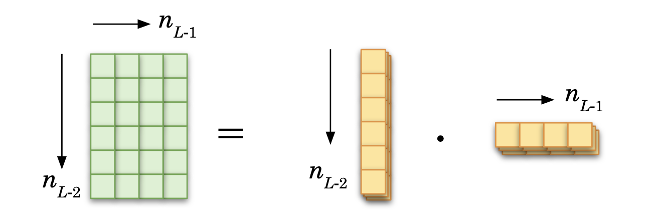
We can rewrite the equations (101) using all the information. The matrix multiplication will be written with the ‘\(\cdot\)’ symbol and element-wise multiplication (applied on vectors) as \(\odot\).

Thus for the last layer, the error is:

(114)\[\qquad \; \boldsymbol{\delta}^{(i,L)}_{1 \times n_L} =\; L^{\prime}\left(\boldsymbol{a}^{(i,L)}_{1 \times n_L}\right) \odot f^{\prime}\left(\boldsymbol{z}^{(i,L)}_{1 \times n_L}\right) \]

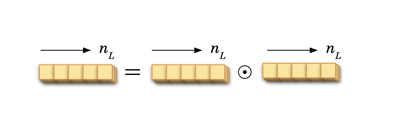
It is an element-wise multiplication of two row vectors. The schematics on top of the equation shows the dimension of the terms. As they are lists with a value for each data sample, and we already use the left/right and up/down directions for matrix and vector operations, the \(i\) index is here the ‘depth’. In the schematics, it is represented as piled up Tetris-like tetrominos; here only a few data samples (sheets) are represented for illustrative purposes.

The derivative of the cost is:

 

(115)\[\qquad \qquad \; \frac{\partial \text {Cost}}{\partial W^{(L)}_{n_{L-1} \times n_{L}}} = \; \frac{1}{m} \; \sum_{i=1}^m \; \left(\boldsymbol{a}^{(i,L-1)}_{1 \times n_{L-1}}\right)^T \cdot \boldsymbol{\delta}^{(i,L)}_{1 \times n_L} \]

 
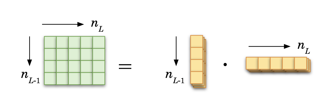
Dimension-wise, the partial derivatives of the cost should be of the same size of the associated weight matrix, as it will be substracted from that weight matrix. So it makes sense in the end to have a matrix created. It is done via the product of a column vector (recall the derivative turns row into column vectors) times a row vector.
 

For the before-last layer, the error is:

 

(116)\[\qquad \qquad \boldsymbol{\delta}^{(i,L-1)}_{1 \times n_{L-1}} = \; \left[ \; \boldsymbol{\delta}^{(i,L)}_{1 \times n_L} \cdot\; \left(W^{(L)}_{n_{L-1} \times n_{L}} \right)^T \right] \odot\; f'\left(\boldsymbol{z}^{(i,L-1)}_{1 \times n_{L-1}}\right) \]

 

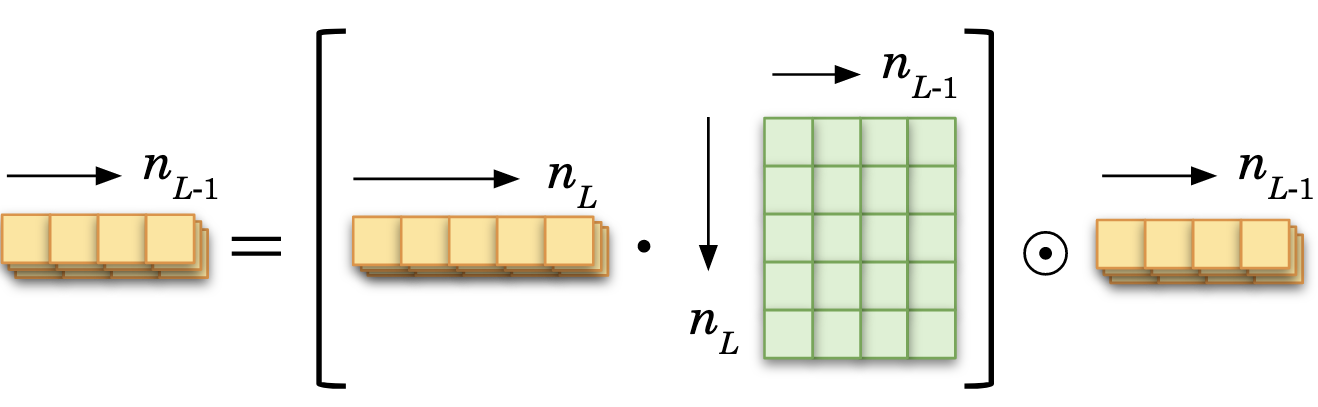
The derivatives of the cost is thus:

 

(117)\[\qquad \qquad \frac{\partial \text {Cost}}{\partial W^{(L-1)}_{n_{L-2} \times n_{L-1}}} = \; \frac{1}{m} \; \sum_{i=1}^m \; \left(\boldsymbol{a}^{(i,L-2)}_{1 \times n_{L-2}}\right)^T \cdot \boldsymbol{\delta}^{(i,L-1)}_{1 \times n_{L-1}} \]

 

That’s it for the math.

 

Now you know how neural networks are trained!

In the assignment, you will code yourself a small neural network from scratch. Don’t worry: it will be guided. In the next lecture, we will see a much more convenient way to build a neural network using dedicated libraries. We will introduce further optimization techniques proper to deep learning.

Exercise

Now that you know the backpropagation algorithm, a question regarding the neural network initialization: what if all weights are first set to the same value? (not zero, as we saw, but any other constant)

Check your answer

If the weights and biases are initialized to the same constant values \(w\) and \(b\), all activation units in a given layer will get the same signal \(a = \sum_{j} w_j \; x_j + b\). As such, all nodes for that layer will be identical. Thus the gradients will be updated the same way. Despite having many neurons per layer, the network will act as if it had only one neuron per layer. Therefore, it is likely to fail to reproduce complex patterns from the data; it won’t be that smart. For a feedforward neural network to work, there should be an asymmetric configuration for it to use each activation unit uniquely. This is why weights and biases should be initalized with random value to break the symmetry.

  

Learn more

The paper that popularized backpropagation, back in 1989:
D. Rumelhart, G. Hinton and R.Williams, Learning representations by back-propagating errors

Some good refresher:
Derivative of the chain rule on math.libretexts.org

Backpropagation explanation with different notation and a source of inspiration (thanks) from ml-cheatsheet