Feedforward Propagation

What is Feedforward Propagation?

It is a first step in the training of a neural network (after initialization of the weights, which will be covered in the next lecture). The forward direction means going from input to output nodes.

Definition 56

The Feedforward Propagation, also called Forward Pass, is the process consisting of computing and storing all network nodes’ output values, starting with the first hidden layer until the last output layer, using at start either a subset or the entire dataset samples.

Forward propagation thus leads to a list of the neural network predictions for each data instance row used as input. At each node, the computation is the key equation (48) we saw in the previous Section Model Representation, written again for convenience:

(55)$$y=f(\sum _{j=1}^n{w}_j{x}_j+b)$$

But there will be some change in the notations. Let’s define everything in the next subsection.

Notations

Let’s say we have the following network with $x_n$ input features, one first hidden layer with $q$ activation units and a second one with $r$ activation units. For simplicity, we will choose an output layer with only one node:

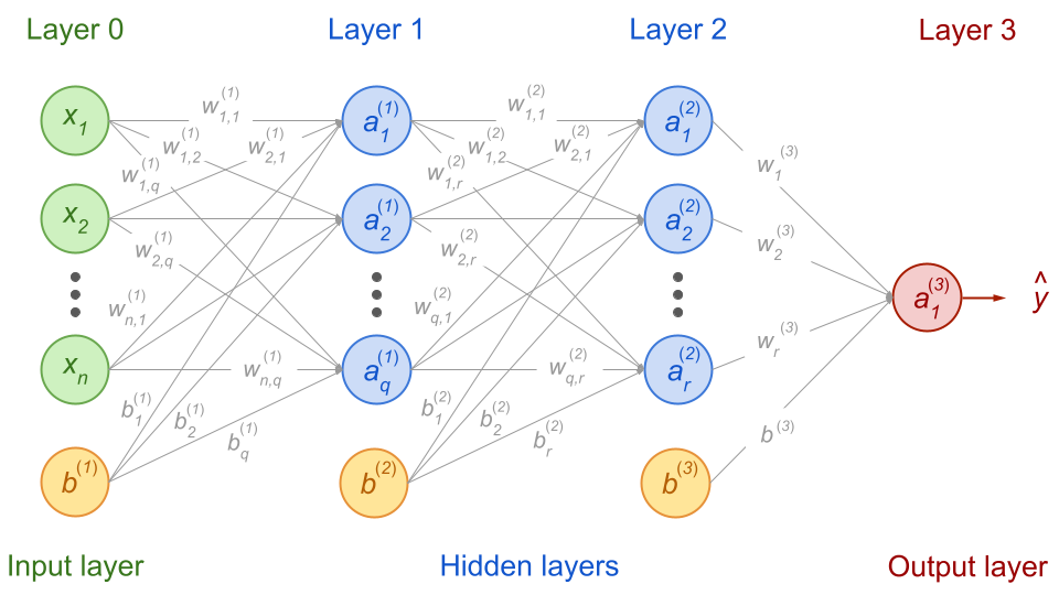
Fig. 53 . A feedforward neural network with the notation we will use for the forward propagation equations (more in text).
_{Image from the author}

There are lots of subscripts and upperscripts here. Let’s explain the conventions we will use.

Input data
We saw in Lecture 2 that the dataset in supervised learning can be represented as a matrix $X$ of $m$ data instances (rows) of $n$ input features (columns). For clarity in the notations, we will focus for now on only one data instance, the $i$th sample row ${\mathit{x}}^{\mathbf{(}\mathit{i}\mathbf{)}}=(x_1,x_2,\cdots ,x_n)$. And we will omit the $(i)$ upperscript for now.

The layer numbering starts at the first hidden layer where $\ell =1$. The input layer is $\ell =0$.

Activation units
In a given layer $\ell =1,2,\cdots ,N^{\text{layer}}$, the activation units will give outputs that we will note as a row vector

$${\mathit{a}}^{\mathbf{(}\mathit{\ell }\mathbf{)}}=(a_1^{(\ell )},a_2^{(\ell )},\cdots ,a_q^{(\ell )}),$$

where the upperscript is the layer number and the subscript is the row of the activation unit in the layer, starting from the top.

Biases
The biases are also row vectors, one for each layer it connects to and of dimension the number of nodes in that layer:

$${\mathit{b}}^{\mathbf{(}\mathit{\ell }\mathbf{)}}=(b_1^{(\ell )},b_2^{(\ell )},\cdots ,b_q^{(\ell )})$$

If the last layer is only made of one node like in our example above, then $b$ is a scalar.

Weights
Now the weights. You may see in the literature different ways to represent them. In here we use a convention we could write as:

$$w_{(\ell -1)\to \ell }^{\ell }$$

In other words, the first index is the row of the node from the previous layer (departing node of the weight’s arrow) and the second index is the row of the node from the current layer (the one the weight’s arrow points to). For instance $w_{3,1}^{(2)}$ is the weight from the third node of layer (1) going to the first node of layer (2).

We can actually represent each weight from layer $\ell -1$ to layer $\ell$ as a matrix $W^{(\ell )}$. If the previous layer $\ell -1$ has $n$ nodes and the layer $\ell$ has $q$ activation units, we will have:

(56)$$\begin{array}{r}{W}^{(\ell )}=\left(\begin{array}{cccc}{w}_{1,1}^{(\ell )}& w_{1,2}^{(\ell )}& \cdots & w_{1,q}^{(\ell )}\\ w_{2,1}^{(\ell )}& w_{2,2}^{(\ell )}& \cdots & w_{2,q}^{(\ell )}\\ ⋮& ⋮& \ddots & ⋮\\ w_{n,1}^{(\ell )}& w_{n,2}^{(\ell )}& \cdots & w_{n,q}^{(\ell )}\end{array}\right)\end{array}$$

Let’s now see how we calculate all the values of the activation units!

Step by step calculations

Computation of the first hidden layer

Let’s use Equation (55) to compute the activation unit outputs of the first layer. The activation function is represented as $f$ here:

(57)$$\begin{array}{r}\begin{array}{rl}{a}_1^{(1)}& =f(w_{1,1}^{(1)}{x}_1+w_{2,1}^{(1)}{x}_2+\cdots +w_{n,1}^{(1)}{x}_n+b_1^{(1)})\\ a_2^{(1)}& =f(w_{1,2}^{(1)}{x}_1+w_{2,2}^{(1)}{x}_2+\cdots +w_{n,2}^{(1)}{x}_n+b_2^{(1)})\\ & ⋮\\ a_q^{(1)}& =f(w_{1,q}^{(1)}{x}_1+w_{2,q}^{(1)}{x}_2+\cdots +w_{n,q}^{(1)}{x}_n+b_q^{(1)})\end{array}\end{array}$$

We can actually write it in the matrix form. Let’s first write it in an expanded version with the matrix elements:

(58)$$\begin{array}{r}{\mathit{a}}^{\mathbf{(}\mathbf{1}\mathbf{)}}=f[(x_1,x_2,\cdots ,x_n)\left(\begin{array}{cccc}{w}_{1,1}^{(1)}& w_{1,2}^{(1)}& \cdots & w_{1,q}^{(1)}\\ w_{2,1}^{(1)}& w_{2,2}^{(1)}& \cdots & w_{2,q}^{(1)}\\ ⋮& ⋮& \ddots & ⋮\\ w_{n,1}^{(1)}& w_{n,2}^{(1)}& \cdots & w_{n,q}^{(1)}\end{array}\right)+(b_1^{(1)},b_2^{(1)},\cdots ,b_q^{(1)})]\end{array}$$

This can be written in a compact way:

(59)$${\mathit{a}}^{\mathbf{(}\mathbf{1}\mathbf{)}}=f(\mathit{x}{W}^{(1)}+{\mathit{b}}^{(1)})$$

Much lighter.

Computation of the second hidden layer

Let’s do the same calculation for the second layer of activation units. Instead of the dataset vector $\mathit{x}$, we will have ${\mathit{a}}^{\mathbf{(}\mathbf{1}\mathbf{)}}$ as input:

(60)$$\begin{array}{r}{\mathit{a}}^{\mathbf{(}\mathbf{2}\mathbf{)}}=f[(a_1^{(1)},a_2^{(1)},\cdots ,a_q^{(1)})\left(\begin{array}{cccc}{w}_{1,1}^{(2)}& w_{1,2}^{(2)}& \cdots & w_{1,r}^{(2)}\\ w_{2,1}^{(2)}& w_{2,2}^{(2)}& \cdots & w_{2,r}^{(2)}\\ ⋮& ⋮& \ddots & ⋮\\ w_{q,1}^{(2)}& w_{q,2}^{(2)}& \cdots & w_{q,r}^{(2)}\end{array}\right)+(b_1^{(2)},b_2^{(2)},\cdots ,b_r^{(2)})]\end{array}$$

And the elegant, light version:

(61)$${\mathit{a}}^{\mathbf{(}\mathbf{2}\mathbf{)}}=f({\mathit{a}}^{\mathbf{(}\mathbf{1}\mathbf{)}}{W}^{(2)}+{\mathit{b}}^{(2)})$$

We start seeing a pattern here thanks to the matricial form. More on this soon in Section General rule for Forward Propagation. Let’s finish the process with the last layer:

Computation of the third hidder layer

With one output node, it is actually simpler than for the hidden layers above. We can still write it in the same form as Equation (61):

(62)$${\mathit{a}}^{\mathbf{(}\mathbf{3}\mathbf{)}}=f({\mathit{a}}^{\mathbf{(}\mathbf{2}\mathbf{)}}{W}^{(3)}+{\mathit{b}}^{(3)})$$

with ${\mathit{a}}^{\mathbf{(}\mathbf{2}\mathbf{)}}=(a_1^{(2)},a_2^{(2)},\cdots ,a_r^{(2)})$ that we calculated above.

In our case ${\mathit{a}}^{\mathbf{(}\mathbf{3}\mathbf{)}}$ has only one element: $a_1^{(3)}=y$.

The matrix $W^{(3)}$ has only one column.

The bias ‘vector’ is actually a scalar: $b^{(3)}$.

That’s the end of the forward propagation process! As you can see, it contains lots of calculations. And now you may understand why activation functions that are simple and fast to compute are preferrable, as they intervene each time we compute the output of an activation unit.

Let’s now generalize this with a general formula.

General rule for Forward Propagation

If we rewrite the first layer of inputs as:

(63)$${\mathit{x}}^{\mathbf{(}\mathit{i}\mathbf{)}}=(x_1,x_2,\cdots ,x_n)=(a_1^{(0)},a_2^{(0)},\cdots ,a_n^{(0)})={\mathit{a}}^{\mathbf{(}\mathbf{0}\mathbf{)}},$$

then we can write a general rule for computing the outputs of a fully connected layer $\ell$ knowing the outputs of the previous layer $\ell$ (which become the layer $\ell$’s inputs):

(64)$${\mathit{a}}^{\mathbf{(}\mathit{\ell }\mathbf{)}}=f({\mathit{a}}^{\mathbf{(}\mathit{\ell }\mathbf{-}\mathbf{1}\mathbf{)}}{W}^{(\ell )}+{\mathit{b}}^{(\ell )})$$

This is the general rule for computing all outputs of a fully connected feedforward neural network.

Summary

Feedforward propagation is the computation of the values of all activation units of a fully connected feedforward neural network.

As the process includes the last layer (output), feedforward propagation also leads to predictions.

These predictions will be compared to the observed values.

Feedforward propagation is a step in the training of a neural network.

The next step of the training is to go ‘backward’, from the output error ${\hat{y}}^{\text{pred}}-y^{\text{obs}}$ to the first layer to then adjust all weights using a gradient-based procedure. This is the core of backpropagation, which we will cover at the next lecture.

Learn More

Very nice animations here illustrating the forward propagation process.
Source: Xinyu You’s course An online deep learning course for humanists