Assignment 3: Neural Network By Hand!
Contents
Assignment 3: Neural Network By Hand!#
In this assignment, you will code a little neural network from scratch! Don’t worry, it will be extremely guided. The two most important points being that you learn and you have fun.
For programmers already fluent in Python
If you have had some programming experience already, please stick to the code template below for grading purposes. Then, feel free to append to your notebook a more elaborate code. And check the bonuses at the end of this assignment!
We want our neural network to solve the XOR problem. This is how the data look like:
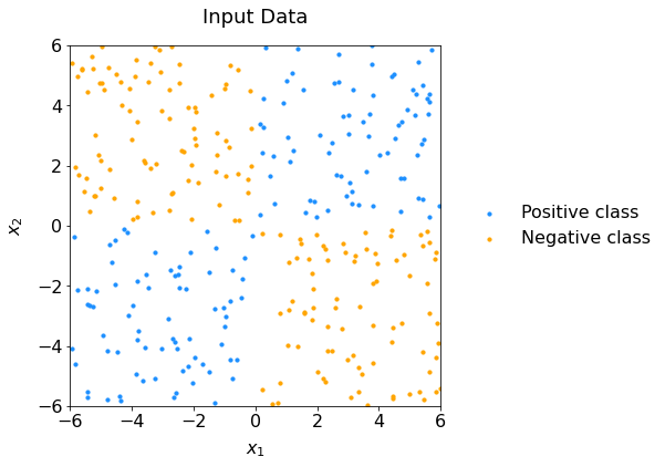
Scatter plot of data representing the XOR configuration: it is not linearly separable.#
Part 1: Derivation of Backpropagation#
In this question, you are asked to derive Equations (100), (108) – (113) from the section on the Backpropagation Algorithm.
Remember that a matrix element \(w_{jk}\) of a matrix \(W\) becomes \(w_{kj}\) once it is transposed as \(W^\top\).
The outer product of two vectors \(a \otimes b\) can also be written as: \(a \; b^\top\) .
Refrain from using indices already taken in the course (\(i\), \(\ell\), \(m\), \(n\)) to avoid confusion with sample index, layer number, total number of samples and number of features, respectively. Lots of other letters are available 😉.
Part 2: Code it!#
Setup#
Copy all of the following into a fresh Jupyter notebook.
import numpy as np
import pandas as pd
import random
import math
np.random.seed(42)

import matplotlib.pyplot as plt
FONTSIZE = 16
params = {
         'figure.figsize' : (6,6),
         'axes.labelsize' : FONTSIZE,
         'axes.titlesize' : FONTSIZE+2,
         'legend.fontsize': FONTSIZE,
         'xtick.labelsize': FONTSIZE,
         'ytick.labelsize': FONTSIZE,
         'xtick.color'    : 'black',
         'ytick.color'    : 'black',
         'axes.facecolor' : 'white',
         'axes.edgecolor' : 'black',
         'axes.titlepad'  :  20,
         'axes.labelpad'  :  10}
plt.rcParams.update(params)

XNAME = 'x1'; XLABEL = r'$x_1$'
YNAME = 'x2'; YLABEL = r'$x_2$'
RANGE = (-6, 6); STEP = 0.1

def predict(output_node, boundary_value):
  output_node.reshape(-1, 1, 1) # a list (m, 1, 1)
  predictions = np.array(output_node > boundary_value, dtype=int)
  return predictions

def plot_cost_vs_iter(train_costs, test_costs, title="Cost evolution"):

  fig, ax = plt.subplots(figsize=(8, 6))
  iters = np.arange(1,len(train_costs)+1)
  ax.plot(iters, train_costs, color='red', lw=1, label='Training set')
  ax.plot(iters, test_costs, color='blue', lw=1, label='Testing set')
  ax.set_xlabel("Number of iterations"); ax.set_xlim(1, iters[-1])
  ax.set_ylabel("Cost")
  ax.legend(loc="upper right", frameon=False)
  ax.set_title(title)
  plt.show()


def get_decision_surface(weights, biases, boundary=0.5, range=RANGE, step=STEP):

  # Create a grid of points spanning the parameter space:
  x1v, x2v = np.meshgrid(np.arange(range[0], range[1]+step, step),
                         np.arange(range[0], range[1]+step, step))

  # Stack it so that it is shaped like X_train: (m,2)
  X_grid = np.c_[x1v.ravel(), x2v.ravel()].reshape(-1,2)

  # Feedforward on all grid points and get binary predictions:
  output = feedforward(X_grid, weights, biases)[-1] # getting only output node
  Ypred_grid = predict(output, boundary)

  return (x1v, x2v, Ypred_grid.reshape(x1v.shape))


def plot_scatter(sig, bkg, ds=None, xname=XNAME, xlabel=XLABEL, yname=YNAME, ylabel=YLABEL, range=RANGE, step=STEP, title="Scatter plot"):

  fig, ax = plt.subplots()

  # Decision surface
  if ds:
    (xx, yy, Z) = ds # unpack contour data
    cs = plt.contourf(xx, yy, Z, levels=[0,0.5,1], colors=['orange','dodgerblue'], alpha=0.3)

  # Scatter signal and background:
  ax.scatter(sig[xname], sig[yname], marker='o', s=10, c='dodgerblue', alpha=1, label='Positive class')
  ax.scatter(bkg[xname], bkg[yname], marker='o', s=10, c='orange',     alpha=1, label='Negative class')

  # Axes, legend and plot:
  ax.set_xlim(range); ax.set_xlabel(xlabel)
  ax.set_ylim(range); ax.set_ylabel(ylabel)

  ax.legend(bbox_to_anchor=(1.04, 0.5), loc="center left", frameon=False)
  ax.set_title(title)
  plt.show()
1. Get the data#
1.1: Get the data file
Retrieve the files of this folder and read them into dataframes train and test.
How many samples are there in each? Write a full sentence to express your answer.
What is the name of the column containing the labels? What are the class values?
1.2: Split signal vs background
Create a sig and bkg dataframes that collect the real signal and value samples.
Hint: this has been done in Tutorial 2.
1.3: Dataframe to NumPy
Declare the following variables to store the dataset into NumPy arrays:
inputs = ['x1', 'x2']
X_train =
y_train =

X_test =
y_test =
2. Functions#
2.1: Weighted Sum
Create the function z that compute the weighted sum of a given activation unit, as seen in class. You do not have to worry about the dimensions of objects here, this will come later. Make sure the names of the arguments are self-explanatory:
def z( ... , ... , ... ):
    # ...
    return #...
2.2: Activation Functions and Derivatives
Write the hyperbolic tan and sigmoid activation functions, followed by their derivatives:
def tanh(z):
    return #...

def sigmoid(z):
    return #...

def sigmoid_prime(z):
    return #...

def tanh_prime(z):
    return #...
2.3: Cross-entropy cost function
Write the cross-entropy cost function.
Hint: It was done in assignment 1
def cross_entropy_cost(y_preds, y_vals):
    #...
    return #...
2.4: Derivative of the Loss
As seen in class, the loss function for classification is defined as:
Find the expression of:
Use a text cell and LaTeX. If you are new to LaTeX, this application will help.
Once you have an expression for the derivative of the loss, code it in python:
def L_prime(y_preds, y_obs):
    return #...
3. Feedforward#
It is time to write the feedforward function! Some information about the network:
The network has two hidden layers
The nodes of the hidden layers use the hyperbolic tangent as activation function
The output layer uses the sigmoid function
3.1: Feedforward Propagation
We do not have to know the number of activation units in each layer as the code here is made to be general. The weights and biases are given as input, stored in lists. Again, you do not have to worry about the indices yet (and I have simplified it by reshaping the input data for you).
Complete the function below that does the feedforward propagation of the network, using the equations shown in class. Look at the output to see how to name your variables!
def feedforward(input_X, weights, biases):

  W1, W2, W3 = weights ; b1, b2, b3 = biases

  m  = len(input_X)
  a0 = input_X.reshape((m, -1, 1))

  # First layer
  #...
  #...

  # Second layer
  #...
  #...

  # Third layer
  #...
  #...

  nodes = [a0, z1, a1, z2, a2, z3, a3]

  return nodes
Check Point
At that point in the assignment, it is possible to ask for a checkup with the instructor before moving forward to …the backward pass (pun intended). Send an email to the instructor with the exact title “[Intro to ML 2024] Assignment 3 Check 1” where you paste the code of the function above (do not send any notebook).
3.2: Predict
This function is given (at the Setup step), yet there is a question for you:
What is the
output_nodein the context of our 2-hidden-layered neural network?What type of values does the function
predictreturn?After successfully executing the
feedforwardfunction, how would you call the functionpredict?
Make sure your explanations are concise yet clear.
4. Neural Network Training#
Time to train! The code below is a skeleton. You will have to complete it. To help you further, hyperparameters are given. You should replace the #... with your own code.
# Hyperparameters
alpha = 0.03
N = 1000 # epochs

# Initialization
m = len(X_train)     # number of data samples
n = X_train.shape[1] # number of input features
q = 3 # number of nodes in first hidden layer
r = 2 # number of nodes in second hidden layer

# WEIGHT MATRICES + BIASES
W1 =  #...
W2 =  #...
W3 =  #...
b1 =  #...
b2 =  #...
b3 =  #...

# OUTPUT LAYER
y_train = np.reshape(y_train, (-1, 1, 1))
y_test  = np.reshape(y_test , (-1, 1, 1))

# Storing cost values for train and test datasets
costs_train = []
costs_test  = []
debug = False

print("Starting the training\n")

# -------------------
#   Start iterations
# -------------------
for t in range(1, N+1):

  # FORWARD PROPAGATION
  # Feedforward on test data:
  nodes_test =  #...
  ypreds_test =  #...

  # Feedforward on train data:
  a0, z1, a1, z2, a2, z3, a3 = #...
  ypreds_train =  #...

  # Cost computation and storage
  J_train = cross_entropy_cost(ypreds_train, y_train)
  J_test  = cross_entropy_cost(ypreds_test,  y_test )
  costs_train.append(J_train)
  costs_test.append(J_test)

  if (t<=100 and t % 10 == 0) or (t>100 and t % 100 == 0):
      print(f"Iteration {t}\t Train cost = {J_train:.4f}  Test cost = {J_test:.4f}   Diff = {J_test-J_train:.5f}")

  # BACKWARD PROPAGATION
  # Errors delta:
  delta_3 = #...
  delta_2 = #...
  delta_1 = #...

  # Partial derivatives:
  dCostdW3 = #...
  dCostdW2 = #...
  dCostdW1 = #...
  dCostdb3 = #...
  dCostdb2 = #...
  dCostdb1 = #...

  if debug and t<3:
    print(f"a0: {a0.shape} a1: {a1.shape} a2: {a2.shape} a3: {a3.shape} ")
    print(f"W3: {W3.shape} z1: {z1.shape} z2: {z2.shape} z3: {z3.shape} ")
    print(f"dCostdW3: {dCostdW3.shape} dCostdW2: {dCostdW2.shape} dCostdW1: {dCostdW1.shape}")

  # Update of weights and biases
  W3 = #...
  W2 = #...
  W1 = #...
  b3 = #...
  b2 = #...
  b1 = #...

print(f'\nEnd of gradient descent after {t} iterations')
Hints (lots of)
Hints on weight initialization
The weight matrices and bias vectors can be simply initialized with a random number between 0 and 1. Use:
an_i_by_j_matrix = np.random.random(( i , j ))
The double parenthesis is important to get the correct shape. To make your code modular, use the variables encoding the number of activation nodes on the first and second hidden layers.
Feedforward and predict
To return the last element of a list:
my_list[-1]
Matrix/Vector Operations
In python the matrix multiplication is done using
@The element-wise multiplication is done using
*
Transpose
To transpose a matrix M:
M.TTo transpose 3D arrays, the indices to reorder are indicated as argument:
np.transpose(my3Darray, (0, 2, 1))will transpose the two last dimensions.
Summing
To sum a 3D array on the first index:
np.sum(my3Darray, axis=0)
5. Plots#
5.1: Cost evolution
Call the provided function to plot the cost evolution of both the training and testing sets.
5.2: Scatter Plot
Use the get_decision_surface and plot_scatter functions to visualize the decision boundaries of your trained neural network. Did your neural network successfully learn the XOR function?
If all goes well, you should obtain something like this:
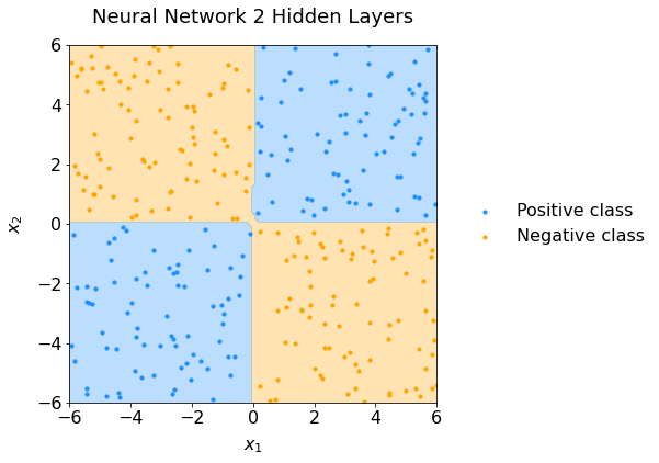
Scatter plot of data representing the XOR configuration and the neural network performance.#
Warning
This assignment is individual. The instructor will be available to answer questions per email and/or during special session. If you are stuck, it is possible to get some elements of answer from the instructor only.
Important
You can use the internet such as the official pages of relevant libraries, forum websites to debug, etc. You can use ChatGPT to help you locally with any python difficulties, but you cannot submit this entire assignment to the bot (and that will not even work).
The instructor and tutors are available throughout the week to answer your questions. Write an email with your well-articulated question(s). The more specific you are in your request, the best we can help you.
Thank you and do not forget to have fun while coding!
Bonuses#
You are done already with time at hand? Great. There is more for you! You can make your network better:
Generalize the computations for any fully connected feedforward network.
Wrap your network in a class (keep it simple: we are not asking to recreate PyTorch here).
Test your network with fancier data, for instance the double spiral! Dataset provided upon request.
Experiment advanced techniques such as momentum and a moving exponential average on the gradients. Does it help? Illustrate with visuals.
Explore whatever you want with your new NN-animal. Have fun!