Assignment 1: Classifier By Hand
Contents
Assignment 1: Classifier By Hand#
In this assignment, you learn step by step how to code a binary classifier by hand!
Don’t worry, it will be guided through.
Introduction: calorimeter showers#
A calorimeter in the context of experimental particle physics is a sub-detector aiming at measuring the energy of incoming particles. At CERN Large Hadron Collider, the giant multipurpose detectors ATLAS and CMS are both equipped with electromagnetic and hadronic calorimeters. The electronic calorimeter, as its name indicates, is measuring the energy of incoming electrons. It is a destructive method: the energetic electron entering the calorimeter will interact with its dense material via the electromagnetic force. It eventually results in the generation of a shower of particles (electromagnetic shower), with a characteristic average depth and width. The depth is along the direction of the incoming particle and the width is the dimension perpendicular to it.
Problem? There can be noisy signals in electromagnetic calorimeters that are generated by hadrons, not electrons.
Your mission is to help physicists by coding a classifier to select electron-showers (signal) from hadron-showers (background).
To this end, you are given a dataset of shower characterists from previous measurements where the incoming particle was known. The main features are the depth and the width.
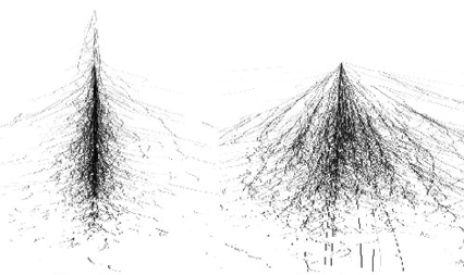
Visualization of an electron shower (left) and hadron shower (right).
From ResearchGate#
Hadron showers are on average longer in the direction of the incoming hadron (depth) and large in the transverse direction (width).
1. Get the Data#
Download the dataset and put it on your GDrive. Open a new Jupyter-notebook from Google-Colab. To mount your drive:
from google.colab import drive
drive.mount('/content/gdrive')
For the following, import the NumPy and pandas libraries:
import sys, os
import numpy as np
import pandas as pd
1.1 Get and load the data
Read the dataset into a dataframe df. What are the columns? Which column stores the labels (targets)?
1.2 How many samples are there?
2. Feature Scaling#
2.1 Explain
If the parameters are initialized randomly between 0 and 1 and the data are not zero-centered, what happens to the gradient descent? Explain the behaviour.
2.2 Standardization
Create for each input feature an extra column in the dataframe to rescale it to a distribution of zero-mean and unit-variance. To see statistical information on a dataframe, a convenient method is:
df.describe()
We will take \(x_1\) and \(x_2\) in the order of the dataframe’s columns. By searching in the documentation for methods retrieving the mean and standard deviation, complete the following code:
MEAN_X1  =
SIGMA_X1 =
MEAN_X2  =
SIGMA_X2 =

df['shower_depth_scaled'] =
df['shower_width_scaled'] =
Hint: recall Definition 12 and the equation to scale a feature according to the standardization method.
Check your results by calling df.describe() on the updated dataframe.
3. Data Prep#
Let’s make the dataset ready for the classifier. As seen in class, the hypothesis function in the linear assumption has the dot product \(\sum_{j=0}^n x^{(i)}_j \theta_j = x^{(i)} \theta^{\; T}\), where by convention \(x_0 = 1\). With 2 input features, there are two parameters to optimize for each feature and the intercept term \(\theta_0\). To perform the dot product above, let’s add to the dataframe a column:
3.1 Adding x0 column
Add a column x0 to the dataframe df filled entirely with ones.
3.2 Matrix X
Create a new dataframe X that contain the x0 column and the columns of the two scaled input features.
3.3 Labels to binary
The target column contains alphabetical labels. Create an extra column in your dataframe called y containing 1 if the sample is an electron shower and 0 if it is a hadron one.
Hint: you can first create an extra column full of 0, then apply a filter using the .loc property from DataFrame. It can be in the form:
df.loc[ CONDITION, COLUMN_TO_UPDATE] = VALUE
Read the pandas documentation on .loc.
3.4 Vector y
Extract from the dataframe this y column with the binary labels in a separate dataframe y.
4. DataFrames to Numpy#
The inputs are almost ready, yet there are still some steps. As we saw in Lecture 3 in Part Performance Metrics, we need to split the dataset in a training and a testing sets. We will use the very convenient train_test_split method from Sciki-Learn. Then, we convert the resulting dataframes to NumPy arrays. This Python library is the standard in data science. In this assignment, you will manipulate NumPy arrays and build the foundations you need to master the programming aspect of machine learning.
Copy this code into your notebook:
from sklearn.model_selection import train_test_split

X_train_df, X_test_df, y_train_df, y_test_df = train_test_split( X, y, test_size=0.2, random_state=42)

X_train = X_train_df.to_numpy() ; y_train = y_train_df.to_numpy()
X_test  = X_test_df.to_numpy()  ; y_test  = y_test_df.to_numpy()
4.1 Shapes
Show the dimensions of the four NumPy arrays using the .shape property. Comment the numbers with respect to the notations defined in class. Does it make sense?
4.2 Test size
Looking at the shapes, explain what test_size represents.
5. Useful Functions#
We saw a lot of functions in the lectures: hypothesis, logistic, cost, etc. We will code these functions as python functions to make the code more modular and easier to read.
Warning
In the following you will work with two dimensional NumPy arrays. Make sure the objects you declare in the code have the correct dimension (number of rows and number of columns).
To help you, look at the examples below.
This creates a 2 x 3 matrix:
>>> a = np.array([[1, 2, 3], [4, 5, 6]])
>>> a
array([[1, 2, 3],
       [4, 5, 6]])
>>> a.shape
(2, 3)
This is a list:
>>> b = [1, 2, 3]
>>> type(b)
<class 'list'>
This makes a 1D NumPy array:
>>> b = np.array([1, 2, 3])
>>> b.shape
(3,)
This declares a 2D NumPy array with one row (aka arow vector):
>>> c = np.array([[1, 2, 3]])
>>> c
array([[1, 2, 3]])
>>> c.shape
(1, 3)
5.1 Linear Sum
Write a function computing the linear sum of the features \(X\) with the \(\boldsymbol{\theta}\) parameters for each input sample.
def lin_sum(X, thetas):

  # Your code here
What should be the dimensions of the returned object? Make sure your function returns a 2D array with the correct shape.
5.2 Logistic Function
Write a function computing the logistic function:
def sigmoid(z):

  # Your code here
5.3 Hypothesis Function
Using the two functions above, write the hypothesis function \(h_\theta(\boldsymbol{x^{(i)}})\):
def h_class(X, thetas):

  # Your code here
5.4 Partial Derivatives of Cross-Entropy Cost Function
In the linear assumption where \(z(\boldsymbol{x^{(i)}}) = \sum_{j=0}^n \theta_j x^{(i)}_j\), the partial derivatives of the cross-entropy cost function are:
Write a function that takes three column vectors (m \(\times\) 1) and computes the partial derivatives \(\frac{\partial}{\partial \theta_j} J(\theta)\) for a given feature \(j\):
def derivatives_cross_entropy(y_preds, y_obs, x_feature):

  # Your code here
Hint: perform an array operation to store all the derivatives in a column vector. Then sum over the elements of that vector. At the end your function should return a scalar, i.e. one value.
5.5 Cross-Entropy Cost Function
Write a function computing the total cost from the 2D column vectors of predictions and observations:
def cross_entropy_cost(y_vals, y_preds):

  # Your code here
6. Classifier#
The core of the action.
Luckily a skeleton is provided. You will have to replace the statments # ... by proper code. It will mostly consist of calling the functions you defined in the previous section.
Test your code frequently. To do so, you can assign dummy temporary values for the variables you do not use yet, so that python knows they are defined and your code can run.
# Hyperparameters
alpha = # ...
N =  # ... epochs

# Number of features + 1 (number of columns in X)
n = # ...

# Initialization of theta *row vector*
thetas = # ...

# Storing cost values for train and test datasets
costs_train = []
costs_test  = []

print("Starting gradient descent\n")

# -------------------
#   Start iterations
# -------------------
for i in range(1, N+1):

  # Get predictions (hypothesis function)
  y_preds = # ...
  y_preds_test = # ...

  # Calculate and store costs with train and test datasets
  J_train = cross_entropy_cost(y_train, y_preds); costs_train.append(J_train)
  J_test  = cross_entropy_cost(y_test, y_preds_test); costs_test.append(J_test)

  # Get partial derivatives d/dTheta_j
  dJ_thetas = np.zeros(shape=(1, n))

  # ...

  # Calculate new theta parameters:
  thetas_new = # ...

  # Update the parameters for the next iteration
  # ...

  # --------------------
  #  P R I N T O U T S
  # --------------------
  # Every 10 iterations and n > 100 every 100 iterations
  if (i<100 and i % 10 == 0) or (i>100 and i % 100 == 0):
    print('[%d]\tt0 = %4.4f  t1 = %4.4f  t2 = %4.4f  Cost = %4.4f  dJ0 = %4.4f  dJ1 = %4.4f  dJ2 = %4.4f' %
         ( i,   thetas[0,0], thetas[0,1], thetas[0,2],   J_train,  dJ_thetas[0,0],   dJ_thetas[0,1],   dJ_thetas[0,2]))

print(f'\nEnd of gradient descent after {i} iterations')

print('Optimized thetas:')
print(f'Theta 0 = {thetas[0,0]:.4f}, Theta 1 = {thetas[0,1]:.4f}, Theta 2 = {thetas[0,2]:.4f}')
If you struggle or cannot finish, summarize in your notebook your trials and investigations.
7. Plot cost versus epochs#
Use the following macro to plot the variation of the total cost vs the iteration number:
def plot_cost_vs_iter(train_costs, test_costs, title="Gradient Descent: Cost evolution"):

  fig, ax = plt.subplots(figsize=(8, 6))

  iters = np.arange(1,len(train_costs)+1)

  ax.plot(iters, train_costs, color='red', lw=1, label='Training set')
  ax.plot(iters, test_costs, color='blue', lw=1, label='Testing set')

  ax.set_xlabel("Number of iterations")
  ax.set_ylabel(r"Cost $J(\theta)$", rotation="horizontal")
  ax.yaxis.set_label_coords(-0.2, 0.5)

  ax.legend(loc="upper right", frameon=False)
  ax.set_title(title, fontsize=18, pad=20)
  plt.show()
Call this macro:
plot_cost_vs_iter(costs_train, costs_test)
You should get something like this:
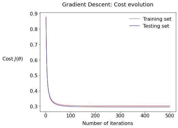
7.1: Describe the plot; what is the fundamental difference between the two series train and test?
7.2: What would it mean if there would be a bigger gap between the test and training values of the cost?
8. Performance#
We will write our own functions to quantitatively assess the performance of the classifier.
Before counting the true and false predictions, we need… predictions! We already wrote a function h_class outputting a prediction as a continuous variable between 0 and 1, equivalent to a probabilitiy. The function below is calling h_class and then fills a python list of binary predictions, so either 0 or 1. For the boundary, recall in the lecture that the sigmoid is symmetric around y = 0.5, so we will work with this boundary for now. Copy this to your notebook:
def make_predictions(thetas, X, y, boundary=0.5):

  bin_preds = [1 if value > boundary else 0 for value in h_class(X, np.array(thetas))[:,0] ]

  return bin_preds
Call the function:
preds = make_predictions(thetas, X_test, y_test, 0.5)
We will work with lists from now on, so flatten the observed test values:
# Turn y_test into 1D array:
obs_test = y_test[:,0]
8.1 Accuracy
Write a function computing the accuracy of the classifier:
def get_accuracy(obs_values, pred_values):

  # Your code here
Call your function using the test set and print the result.
8.2 Recall
def get_recall(obs_values, pred_values):

  # Your code here
Call your function, still with the test set of course, and print the result.
BRAVO! You know now the math behind a binary classifier!
X. BONUS: Decision Boundaries#
This is for advanced programmers and/or your curiosity and/or if you have the time. Bonus points will be given even if you answer with math equations only and not necessarily the associated python code. Of course you if you succeed in getting the python, more bonus points for you!
Goal
We want to draw on a scatter plot the lines corresponding to different decision boundaries.
Tip
Scroll down at the very end to see where we are heading to.
X.0 Scatter plot
The first step is to split the signal and background into two different dataframes. Using the general dataframe df defined at the beginning:
all_sig = df[df['type'] == 'electron'][['shower_depth', 'shower_width']]
all_bkg = df[df['type'] ==  'hadron' ][['shower_depth', 'shower_width']]
The plotting macro:
X1NAME = 'shower_depth'; X1LABEL = 'Shower depth [mm]'
X2NAME = 'shower_width'; X2LABEL = 'Shower width [mm]'
X1MIN  = 0 ; X1MAX = 200
X2MIN  = 0 ; X2MAX =  60

# Raw scatter plot
def plot_scatter(sig, bkg, boundaries=False,
                 x1name=X1NAME, x1label=X1LABEL, x1min=X1MIN, x1max=X1MAX,
                 x2name=X2NAME, x2label=X2LABEL, x2min=X2MIN, x2max=X2MAX,
                 figsize=(6, 6), fontsize=20, alpha=0.2, title="Scatter plot"):

  fig, ax = plt.subplots(figsize=figsize)

  # ------------------
  #      A X E S
  # ------------------
  ax.set(xlim=(x1min, x1max), ylim=(x2min, x2max))
  ax.set_xlabel(x1label); ax.set_ylabel(x2label)

  # ------------------
  #   S C A T T E R
  # ------------------
  scat_el = ax.scatter(sig[x1name], sig[x2name], marker='.', s=1, c='dodgerblue', alpha=alpha)
  scat_had= ax.scatter(bkg[x1name], bkg[x2name], marker='.', s=1, c='darkorange', alpha=alpha)

  # ----------------------
  #  B O U N D A R I E S
  # ----------------------
  #if boundaries:
    # ... stuff to do here

  # ------------------
  #   L E G E N D S
  # ------------------
  # Legend scatter
  h = [scat_el, scat_had]
  legScatter = ax.legend(handles=h, labels=['electron', 'hadron'],
                         title="Shower type\n", title_fontsize=fontsize, markerscale=20,
                         bbox_to_anchor=(1.06, 0.8), loc="center left" , frameon=False)

  # Legend boundary
  if boundaries:
    ax.add_artist(legScatter)
    legLines = ax.legend(title="Decision boundaries",
                       bbox_to_anchor=(1.06, 0.3), loc="center left",
                       title_fontsize=fontsize, frameon=False)

  ax.set_title(title, fontsize=fontsize, pad=20)
  print('\n\n') ; plt.show()
To call it:
plot_scatter(all_sig, all_bkg,
             figsize=(6, 6), fontsize=20, alpha=0.2, title="Calorimeter Showers")
X.1 Useful functions
Recall the logistic function:
Write a function rev_sigmoid that outputs the value \(z = f(\hat{y})\).
Write a function scale_inputs that scales a list of raw input features, either \(x_1\) or \(x_2\), according to the standardization procedure.
Write the function unscale_inputs that does the contrary.
X.2 Equation
For a given threshold \(\hat{y}\), write the equation of the line boundary: \(x_2 = f(\boldsymbol{\theta}, x_1, \hat{y})\).
X.3 Coordinate points
To draw a line on a plot in Matplotlib, one needs to provide the coordinates as a set of two data points.
Write a function that compute the coordinates x2_left and x2_right – associated with the values of x1_min and x1_max respectively – of a decision boundary line at a given threshold \(\hat{y}\). (recall 0.5 is the standard one for logistic regression).
def get_boundary_line_x2(threshold, thetas, x1_min=X1MIN, x1_max=X1MAX):

  # Your code here
Warrior-level bonus: compute this for several thresholds, i.e. the function returns a list of line properties. Tip: it’s convenient to store the result in a dictionary. For instance you can have keys threshold, x2_left, x2_right.
X.4 Plotting the boundaries (advanced)
In the scatter plot code provided, uncomment the boundary section and draw the line(s) using the Matplotlib plot function.
   #...
   ax.plot([x1min, x1max], [x2_left, x2_right], color='r', ls='-', lw=2)
   #...
In the very end, this is how it would render:
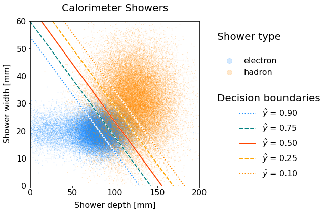
Scatter plot of electron and hadron showers with decision boundary lines for various thresholds.
Code will be shown while releasing solutions.#
The higher the threshold, the more the boundary line shifts downwards in the electron-dense area. Why is that the case?
Important
You are encouraged to work in groups of two, however submissions are individual.
If you have received help from your peers and/or have worked within a group, summarize in the header of your notebook the involved students, how they helped you and the contributions of each group member. This is to ensure fairness in the evaluation.
You can use the internet such as the official pages of relevant libraries, forum websites to debug, etc. However, using an AI such as ChatGPT would be considered cheating (and not good for you anyway to develop your programming skills).
The instructor and tutors are available throughout the week to answer your questions. Write an email with your well-articulated question(s). Put in CC your teammates if any.
Thank you and do not forget to have fun while coding!